pacman::p_load(rgdal, spdep, tmap, sf, ClustGeo,
               ggpubr, cluster, factoextra, NbClust,
heatmaply, corrplot, psych, tidyverse, GGally, funModeling)Take-home_exercise2
Regionalisation of Multivariate Water Point Attributes with Non-spatially Constrained and Spatially Constrained Clustering Methods
Overview
The process of creating regions is called reginalisation. A regionalisation is a special kind of clustering where the objective is to group observations which are similar in their statistical attributes, but also in their spatial location. In this sense, regionalization embeds the same logic as standard clustering techniques, but also applies a series of geographical constraints. Often, these constraints relate to connectivity: two candidates can only be grouped together in the same region if there exists a path from one member to another member that never leaves the region. These paths often model the spatial relationships in the data, such as contiguity or proximity. However, connectivity does not always need to hold for all regions, and in certain contexts it makes sense to relax connectivity or to impose different types of geographic constraints.
The Task
The specific tasks of this take-home exercise are as follows:
Using appropriate sf method, import the shapefile into R and save it in a simple feature data frame format. Note that there are three Projected Coordinate Systems of Nigeria, they are: EPSG: 26391, 26392, and 26303. You can use any one of them.
Using appropriate tidyr and dplyr methods, derive the proportion of functional and non-functional water point at LGA level (i.e. ADM2).
Combining the geospatial and aspatial data frame into simple feature data frame.
Delineating water point measures functional regions by using conventional hierarchical clustering.
Delineating water point measures functional regions by using spatially constrained clustering algorithms.
Data
Aspatial Data
Water point data exchange WPdx+ data set.
Geospatial data
Nigeria Level-2 Administrative Boundary (also known as Local Government Area) polygon features GIS data
Getting Started
Before we get started, it is important for us to install the necessary R packages into R and launch these R packages into R environment.
Spatial data handling
- sf, rgdal and spdep
Attribute data handling
- tidyverse, especially readr, ggplot2 and dplyr
Choropleth mapping
- tmap
Multivariate data visualisation and analysis
- coorplot, ggpubr, and heatmaply
Cluster analysis
cluster
ClustGeo
Setting Up Working Environment
Install sf, tidyverse, tmap, spdep, funModeling packages of R.
Importing Data
Importing Spatial Data
The code chunk below is to import the water point geospatial data into r environment.
wp_nga <- read_csv("Data/WPdx.csv") %>%
  filter(`#clean_country_name` == "Nigeria")
Warning: One or more parsing issues, call `problems()` on your data frame for details,
e.g.:
dat <- vroom(...)
problems(dat)Rows: 406566 Columns: 70
── Column specification ────────────────────────────────────────────────────────
Delimiter: ","
chr (43): #source, #report_date, #status_id, #water_source_clean, #water_sou...
dbl (23): row_id, #lat_deg, #lon_deg, #install_year, #fecal_coliform_value, ...
lgl (4): #rehab_year, #rehabilitator, is_urban, latest_record
ℹ Use `spec()` to retrieve the full column specification for this data.
ℹ Specify the column types or set `show_col_types = FALSE` to quiet this message.wp_nga$Geometry = st_as_sfc(wp_nga$`New Georeferenced Column`)wp_sf <- st_sf(wp_nga, crs=4326)
wp_sfSimple feature collection with 95008 features and 70 fields
Geometry type: POINT
Dimension: XY
Bounding box: xmin: 2.707441 ymin: 4.301812 xmax: 14.21828 ymax: 13.86568
Geodetic CRS: WGS 84
# A tibble: 95,008 × 71
row_id `#source` #lat_…¹ #lon_…² #repo…³ #stat…⁴ #wate…⁵ #wate…⁶ #wate…⁷
* <dbl> <chr> <dbl> <dbl> <chr> <chr> <chr> <chr> <chr>
1 429068 GRID3 7.98 5.12 08/29/… Unknown <NA> <NA> Tapsta…
2 222071 Federal Minis… 6.96 3.60 08/16/… Yes Boreho… Well Mechan…
3 160612 WaterAid 6.49 7.93 12/04/… Yes Boreho… Well Hand P…
4 160669 WaterAid 6.73 7.65 12/04/… Yes Boreho… Well <NA>
5 160642 WaterAid 6.78 7.66 12/04/… Yes Boreho… Well Hand P…
6 160628 WaterAid 6.96 7.78 12/04/… Yes Boreho… Well Hand P…
7 160632 WaterAid 7.02 7.84 12/04/… Yes Boreho… Well Hand P…
8 642747 Living Water … 7.33 8.98 10/03/… Yes Boreho… Well Mechan…
9 642456 Living Water … 7.17 9.11 10/03/… Yes Boreho… Well Hand P…
10 641347 Living Water … 7.20 9.22 03/28/… Yes Boreho… Well Hand P…
# … with 94,998 more rows, 62 more variables: `#water_tech_category` <chr>,
# `#facility_type` <chr>, `#clean_country_name` <chr>, `#clean_adm1` <chr>,
# `#clean_adm2` <chr>, `#clean_adm3` <chr>, `#clean_adm4` <chr>,
# `#install_year` <dbl>, `#installer` <chr>, `#rehab_year` <lgl>,
# `#rehabilitator` <lgl>, `#management_clean` <chr>, `#status_clean` <chr>,
# `#pay` <chr>, `#fecal_coliform_presence` <chr>,
# `#fecal_coliform_value` <dbl>, `#subjective_quality` <chr>, …Importing Water Point Geospatial Data
The chunk below is to import the LGA boundary data into r environment.
nga <- st_read(dsn = "Data",
               layer = "geoBoundaries-NGA-ADM2",
               crs = 4326) %>%
  select(shapeName)
Reading layer `geoBoundaries-NGA-ADM2' from data source
`D:\yuetongz\ISSS624\Take-home_Ex\Take-home_Ex2\Data' using driver `ESRI Shapefile'
Simple feature collection with 774 features and 5 fields
Geometry type: MULTIPOLYGON
Dimension: XY
Bounding box: xmin: 2.668534 ymin: 4.273007 xmax: 14.67882 ymax: 13.89442
Geodetic CRS: WGS 84Data Wrangling
The code chunk below to check shapeName duplicates.
nga <- (nga[order(nga$shapeName), ])

nga<- nga %>%
  mutate(shapeName = tolower(shapeName))

duplicate_Name <- nga$shapeName[ nga$shapeName %in% nga$shapeName[duplicated(nga$shapeName)] ]

duplicate_Name
[1] "bassa" "bassa" "ifelodun" "ifelodun" "irepodun" "irepodun"
[7] "nasarawa" "nasarawa" "obi" "obi" "surulere" "surulere"nga$shapeName[c(94,95,304,305,355,356,518,519,546,547,693,694)] <- c("Bassa (Kogi)","Bassa (Plateau)",
"Ifelodun (Kwara)","Ifelodun (Osun)",
"Irepodun (Kwara)","Irepodun (Osun)",
"Nassarawa (Kano)","Nassarawa",
"Obi (Benue)","Obi(Nasarawa)",
"Surulere (Lagos)","Surulere (Oyo)")
length((nga$shapeName[ nga$shapeName %in% nga$shapeName[duplicated(nga$shapeName)] ]))[1] 0wp_sf <- st_join(wp_sf, nga)The code chunk below renames the columns in wp_sf.
wp_sfT <- wp_sf %>%
  rename ("Country" = "#clean_country_name",
          "clean_adm2" = "#clean_adm2",
          "status" = "#status_clean",
          "lat" = "#lat_deg",
          "long" = "#lon_deg",
          "water_tech" = "#water_tech_category") %>%
  mutate(status = replace_na(status, "Unknown"), water_tech = replace_na(water_tech, "Unknown")) %>%
  select (water_tech,clean_adm2,status,lat,long,usage_capacity, is_urban)
The code chunk below creates water point in functional, non-functional,unknown, hand pump, usage capacity count less than 1000, usage capacity count equal or more than 1000, and rural areas.
functional <- wp_sfT %>%
  filter(`status` %in%  c("Functional", "Functional but not in use" , "Functional but needs repair")) %>%
  select(`lat`, `long`, `water_tech`, `clean_adm2`, `status`, `usage_capacity`, `is_urban`)
nonfunctional <- wp_sfT %>%
filter(`status` %in% c("Abandoned/Decommissioned", "Abandoned", "Non functional due to dry season", "Non-Functional", "Non-Functional due to dry season")) %>%
select(`lat`, `long`, `water_tech`, `clean_adm2`, `status`, `usage_capacity`, `is_urban`)unknown_wp <- wp_sfT %>%
filter(`status` %in% c("Unknown")) %>%
select(`lat`, `long`, `water_tech`, `clean_adm2`, `status`, `usage_capacity`, `is_urban`)handpump_count <- wp_sfT %>%
filter(`water_tech` %in% c("Hand Pump")) %>%
select(`lat`, `long`, `water_tech`, `clean_adm2`, `status`, `usage_capacity`, `is_urban`)usageL1k <- wp_sfT %>%
filter(`usage_capacity` < 1000) %>%
select(`lat`, `long`, `water_tech`, `clean_adm2`, `status`, `usage_capacity`, `is_urban`)usage1k <- wp_sfT %>%
filter(`usage_capacity` == 1000) %>%
select(`lat`, `long`, `water_tech`, `clean_adm2`, `status`, `usage_capacity`, `is_urban`)ruralWP <- wp_sfT %>%
filter(`is_urban` == "FALSE") %>%
select(`lat`, `long`, `water_tech`, `clean_adm2`, `status`, `usage_capacity`, `is_urban`)st_crs(nga)Coordinate Reference System:
User input: EPSG:4326
wkt:
GEOGCRS["WGS 84",
ENSEMBLE["World Geodetic System 1984 ensemble",
MEMBER["World Geodetic System 1984 (Transit)"],
MEMBER["World Geodetic System 1984 (G730)"],
MEMBER["World Geodetic System 1984 (G873)"],
MEMBER["World Geodetic System 1984 (G1150)"],
MEMBER["World Geodetic System 1984 (G1674)"],
MEMBER["World Geodetic System 1984 (G1762)"],
MEMBER["World Geodetic System 1984 (G2139)"],
ELLIPSOID["WGS 84",6378137,298.257223563,
LENGTHUNIT["metre",1]],
ENSEMBLEACCURACY[2.0]],
PRIMEM["Greenwich",0,
ANGLEUNIT["degree",0.0174532925199433]],
CS[ellipsoidal,2],
AXIS["geodetic latitude (Lat)",north,
ORDER[1],
ANGLEUNIT["degree",0.0174532925199433]],
AXIS["geodetic longitude (Lon)",east,
ORDER[2],
ANGLEUNIT["degree",0.0174532925199433]],
USAGE[
SCOPE["Horizontal component of 3D system."],
AREA["World."],
BBOX[-90,-180,90,180]],
ID["EPSG",4326]]st_crs(wp_sfT)Coordinate Reference System:
User input: EPSG:4326
wkt:
GEOGCRS["WGS 84",
ENSEMBLE["World Geodetic System 1984 ensemble",
MEMBER["World Geodetic System 1984 (Transit)"],
MEMBER["World Geodetic System 1984 (G730)"],
MEMBER["World Geodetic System 1984 (G873)"],
MEMBER["World Geodetic System 1984 (G1150)"],
MEMBER["World Geodetic System 1984 (G1674)"],
MEMBER["World Geodetic System 1984 (G1762)"],
MEMBER["World Geodetic System 1984 (G2139)"],
ELLIPSOID["WGS 84",6378137,298.257223563,
LENGTHUNIT["metre",1]],
ENSEMBLEACCURACY[2.0]],
PRIMEM["Greenwich",0,
ANGLEUNIT["degree",0.0174532925199433]],
CS[ellipsoidal,2],
AXIS["geodetic latitude (Lat)",north,
ORDER[1],
ANGLEUNIT["degree",0.0174532925199433]],
AXIS["geodetic longitude (Lon)",east,
ORDER[2],
ANGLEUNIT["degree",0.0174532925199433]],
USAGE[
SCOPE["Horizontal component of 3D system."],
AREA["World."],
BBOX[-90,-180,90,180]],
ID["EPSG",4326]]nga$WPCount <- lengths(st_intersects(nga, wp_sfT))nga$functional <- lengths(st_intersects(nga, functional))nga$nonfunctional <- lengths(st_intersects(nga, unknown_wp))nga$unknown_wp <- lengths(st_intersects(nga, nonfunctional))nga$handpump <- lengths(st_intersects(nga, handpump_count))nga$usage1k <- lengths(st_intersects(nga, usage1k))nga$usageL1k <- lengths(st_intersects(nga, usageL1k))nga$ruralWP <- lengths(st_intersects(nga, ruralWP))nga <- nga %>%
mutate(`pct_functional` = `functional`/`WPCount`) %>%
mutate(`pct_nonfunctional` = `nonfunctional`/`WPCount`) %>%
mutate(`pct_handpump` = `handpump`/`WPCount`) %>%
mutate(`pct_usage1k` = `usage1k`/`WPCount`) %>%
mutate(`pct_usageL1k` = `usageL1k`/`WPCount`) %>%
mutate(`pct_ruralWP` = `ruralWP`/`WPCount`)nga <- nga[-c(3, 86, 241, 250, 252, 261, 400, 406, 447, 473, 492, 507, 526),]nga$`pct_functional`[is.na(nga$`pct_functional`)] <- 0
nga$`pct_nonfunctional`[is.na(nga$`pct_nonfunctional`)] <- 0
nga$`pct_handpump`[is.na(nga$`pct_handpump`)] <- 0
nga$`pct_usage1k`[is.na(nga$`pct_usage1k`)] <- 0
nga$`pct_usageL1k`[is.na(nga$`pct_usageL1k`)] <- 0
nga$`pct_ruralWP`[is.na(nga$`pct_ruralWP`)] <- 0nga_sf <- st_transform(nga, crs = 26391)
st_crs(nga_sf)Coordinate Reference System:
User input: EPSG:26391
wkt:
PROJCRS["Minna / Nigeria West Belt",
BASEGEOGCRS["Minna",
DATUM["Minna",
ELLIPSOID["Clarke 1880 (RGS)",6378249.145,293.465,
LENGTHUNIT["metre",1]]],
PRIMEM["Greenwich",0,
ANGLEUNIT["degree",0.0174532925199433]],
ID["EPSG",4263]],
CONVERSION["Nigeria West Belt",
METHOD["Transverse Mercator",
ID["EPSG",9807]],
PARAMETER["Latitude of natural origin",4,
ANGLEUNIT["degree",0.0174532925199433],
ID["EPSG",8801]],
PARAMETER["Longitude of natural origin",4.5,
ANGLEUNIT["degree",0.0174532925199433],
ID["EPSG",8802]],
PARAMETER["Scale factor at natural origin",0.99975,
SCALEUNIT["unity",1],
ID["EPSG",8805]],
PARAMETER["False easting",230738.26,
LENGTHUNIT["metre",1],
ID["EPSG",8806]],
PARAMETER["False northing",0,
LENGTHUNIT["metre",1],
ID["EPSG",8807]]],
CS[Cartesian,2],
AXIS["(E)",east,
ORDER[1],
LENGTHUNIT["metre",1]],
AXIS["(N)",north,
ORDER[2],
LENGTHUNIT["metre",1]],
USAGE[
SCOPE["Engineering survey, topographic mapping."],
AREA["Nigeria - onshore west of 6°30'E, onshore and offshore shelf."],
BBOX[3.57,2.69,13.9,6.5]],
ID["EPSG",26391]]Exploratory Data Analysis (EDA)
The code chunk below is to display the distribution of status_cle field in wp_nga
freq(data=wp_sfT,
     input = 'status')
Warning: The `<scale>` argument of `guides()` cannot be `FALSE`. Use "none" instead as
of ggplot2 3.3.4.
ℹ The deprecated feature was likely used in the funModeling package.
Please report the issue at <https://github.com/pablo14/funModeling/issues>.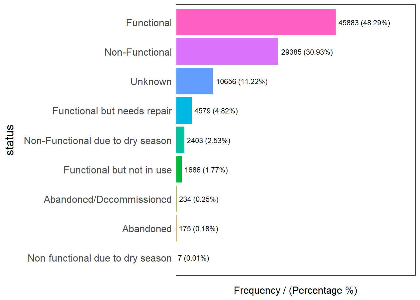
                            status frequency percentage cumulative_perc
1                       Functional     45883      48.29           48.29
2                   Non-Functional     29385      30.93           79.22
3                          Unknown     10656      11.22           90.44
4      Functional but needs repair      4579       4.82           95.26
5 Non-Functional due to dry season      2403       2.53           97.79
6        Functional but not in use      1686       1.77           99.56
7         Abandoned/Decommissioned       234       0.25           99.81
8                        Abandoned       175       0.18           99.99
9 Non functional due to dry season 7 0.01 100.00freq(data=wp_sfT,
input = 'water_tech')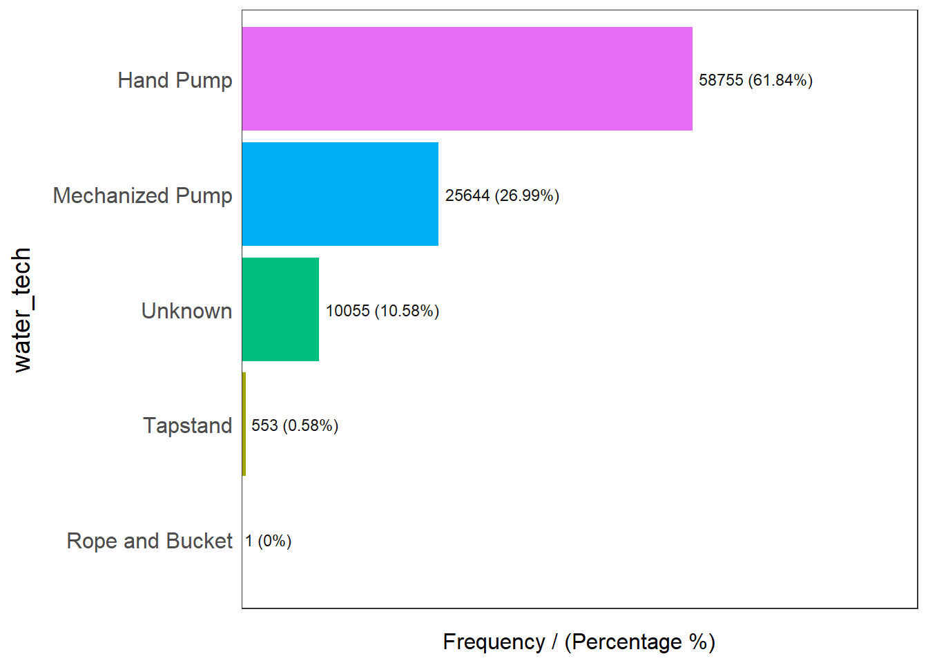
       water_tech frequency percentage cumulative_perc
1       Hand Pump     58755      61.84           61.84
2 Mechanized Pump     25644      26.99           88.83
3         Unknown     10055      10.58           99.41
4        Tapstand       553       0.58           99.99
5 Rope and Bucket 1 0.00 100.00freq(data=wp_sfT,
input = 'is_urban')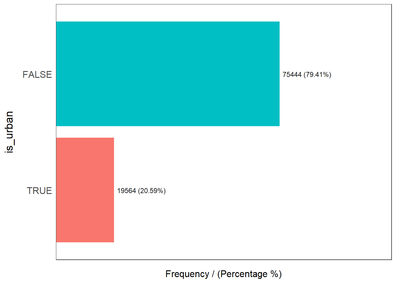
  is_urban frequency percentage cumulative_perc
1    FALSE     75444      79.41           79.41
2     TRUE     19564      20.59          100.00
Plot the histogram and boxplot of functional water point by using the code chunk below.
func_his <- ggplot(data=nga_sf,
             aes(x= pct_functional)) +
  geom_histogram(bins=20,
                 color="black",
                 fill="light blue")

func_box <- ggplot(data=nga_sf,
             aes(x= pct_functional)) +
  geom_boxplot( color="black",
                 fill="light blue")

ggarrange( func_his,func_box,
          ncol = 2)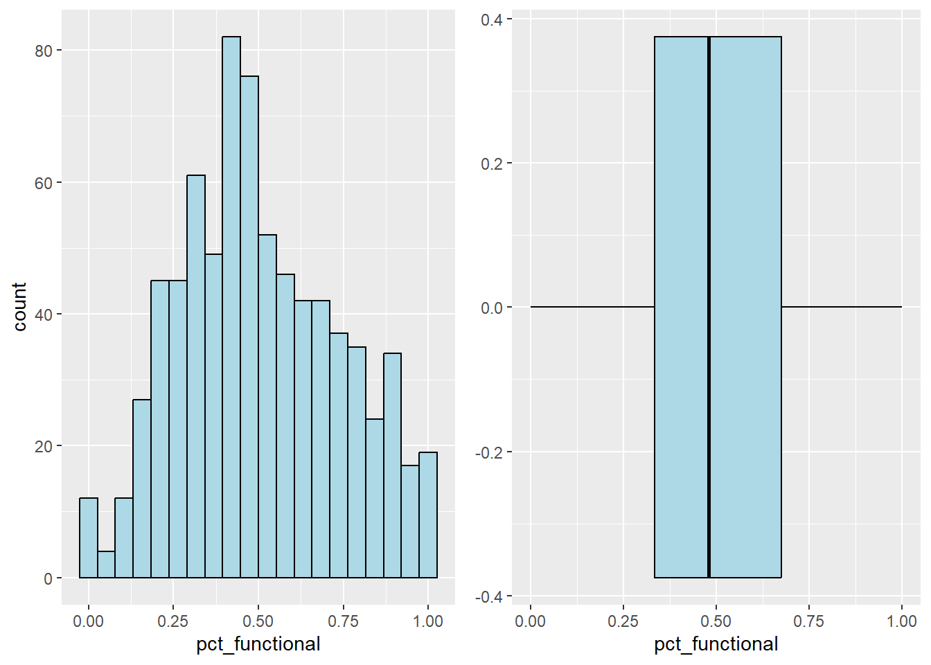
Plot the histogram and boxplot of non-functional water point by using the code chunk below.
non_his <- ggplot(data=nga_sf,
             aes(x= pct_nonfunctional)) +
  geom_histogram(bins=20,
                 color="black",
                 fill="light blue")

non_box <- ggplot(data=nga_sf,
             aes(x= pct_nonfunctional)) +
  geom_boxplot( color="black",
                 fill="light blue")

ggarrange( non_his,non_box,
          ncol = 2)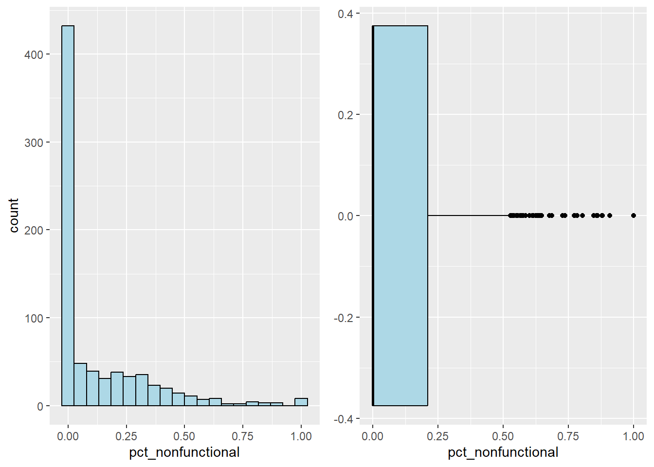
Plot the histogram and boxplot of hand pump water point by using the code chunk below.
hand_his <- ggplot(data=nga_sf,
             aes(x= pct_handpump)) +
  geom_histogram(bins=20,
                 color="black",
                 fill="light blue")

hand_box <- ggplot(data=nga_sf,
             aes(x= pct_handpump)) +
  geom_boxplot( color="black",
                 fill="light blue")

ggarrange( hand_his,hand_box,
          ncol = 2)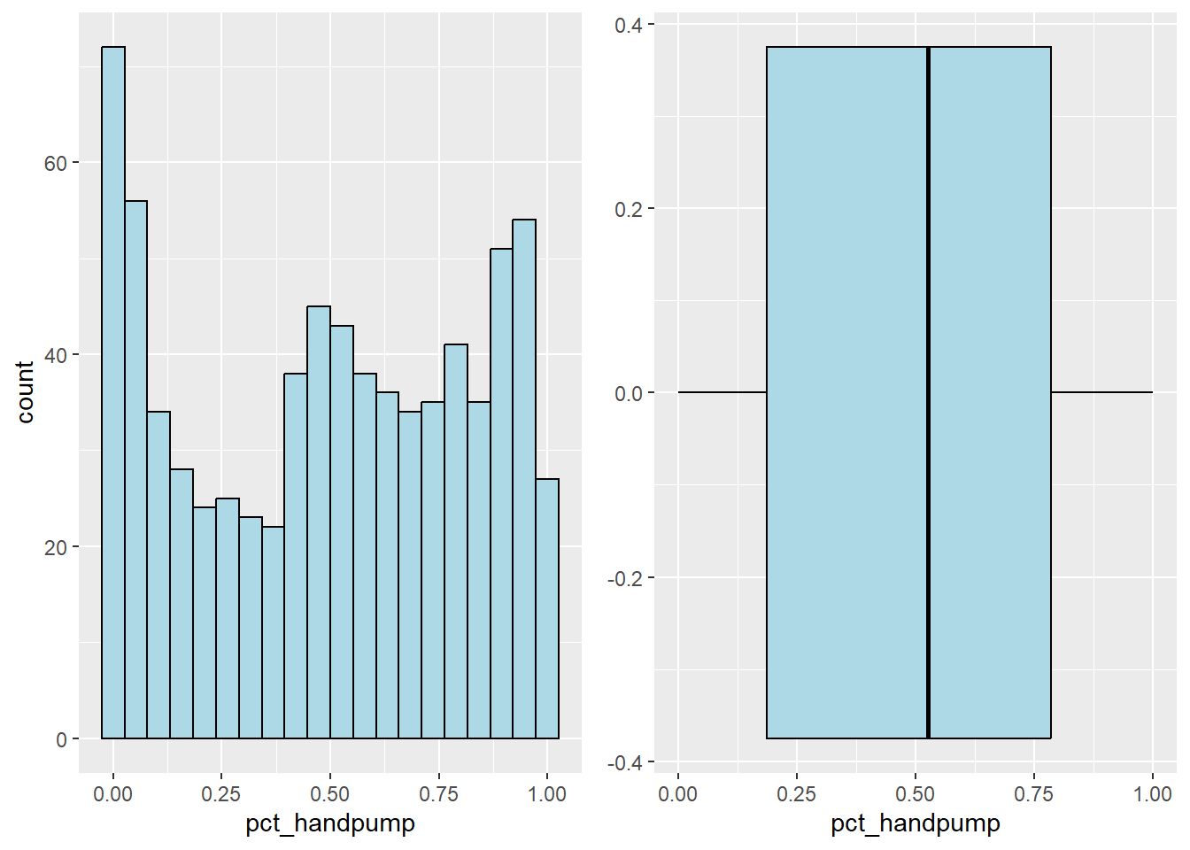
Plot the histogram and boxplot of water point usage capacity equal to or more than 1000 by using the code chunk below.
u1000_his <- ggplot(data=nga_sf,
             aes(x= pct_usage1k)) +
  geom_histogram(bins=20,
                 color="black",
                 fill="light blue")

u1000_box <- ggplot(data=nga_sf,
             aes(x= pct_usage1k)) +
  geom_boxplot( color="black",
                 fill="light blue")

ggarrange( u1000_his,u1000_box,
          ncol = 2)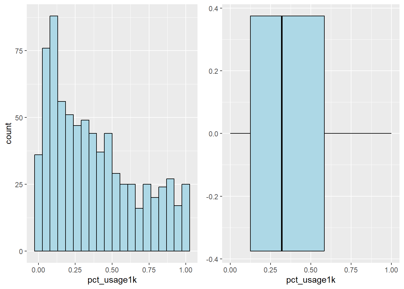
Plot the histogram and boxplot of water point usage capacity less than 1000 by using the code chunk below.
l1000_his <- ggplot(data=nga_sf,
             aes(x= pct_usageL1k)) +
  geom_histogram(bins=20,
                 color="black",
                 fill="light blue")

l1000_box <- ggplot(data=nga_sf,
             aes(x= pct_usageL1k)) +
  geom_boxplot( color="black",
                 fill="light blue")

ggarrange( l1000_his,l1000_box,
          ncol = 2)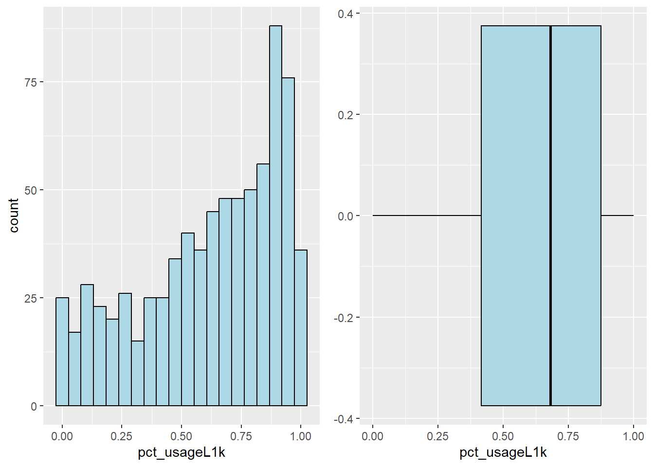
Plot the histogram and boxplot of rural water point by using the code chunk below.
rur_his <- ggplot(data=nga_sf,
             aes(x= pct_ruralWP)) +
  geom_histogram(bins=20,
                 color="black",
                 fill="light blue")

rur_box <- ggplot(data=nga_sf,
             aes(x= pct_ruralWP)) +
  geom_boxplot( color="black",
                 fill="light blue")

ggarrange( rur_his,rur_box,
          ncol = 2)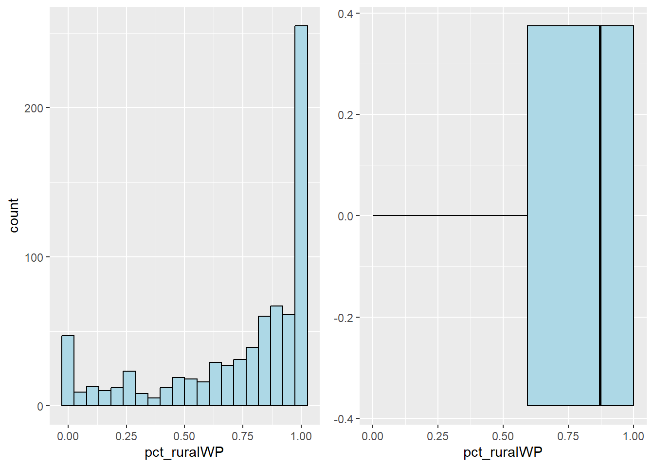
Preparing a choropleth map
Plot the choropleth maps showing the dsitribution of functional, non-functional, hand pump water point, water point of usage capacity less than, equal to and more than 1000, and rural water point by using the code chunk below.
tm_shape(nga_sf) +
    tm_polygons(c("pct_functional", "pct_nonfunctional", "pct_handpump","pct_usage1k","pct_usageL1k", "pct_ruralWP"),
                style="jenks") +
    tm_facets(sync = TRUE, ncol = 3, nrow = 2) +
  tm_legend(legend.position = c("right", "bottom"), legend.title.size = 1.5,legend.text.size = 1)+
  tm_layout(outer.margins=0, asp=0)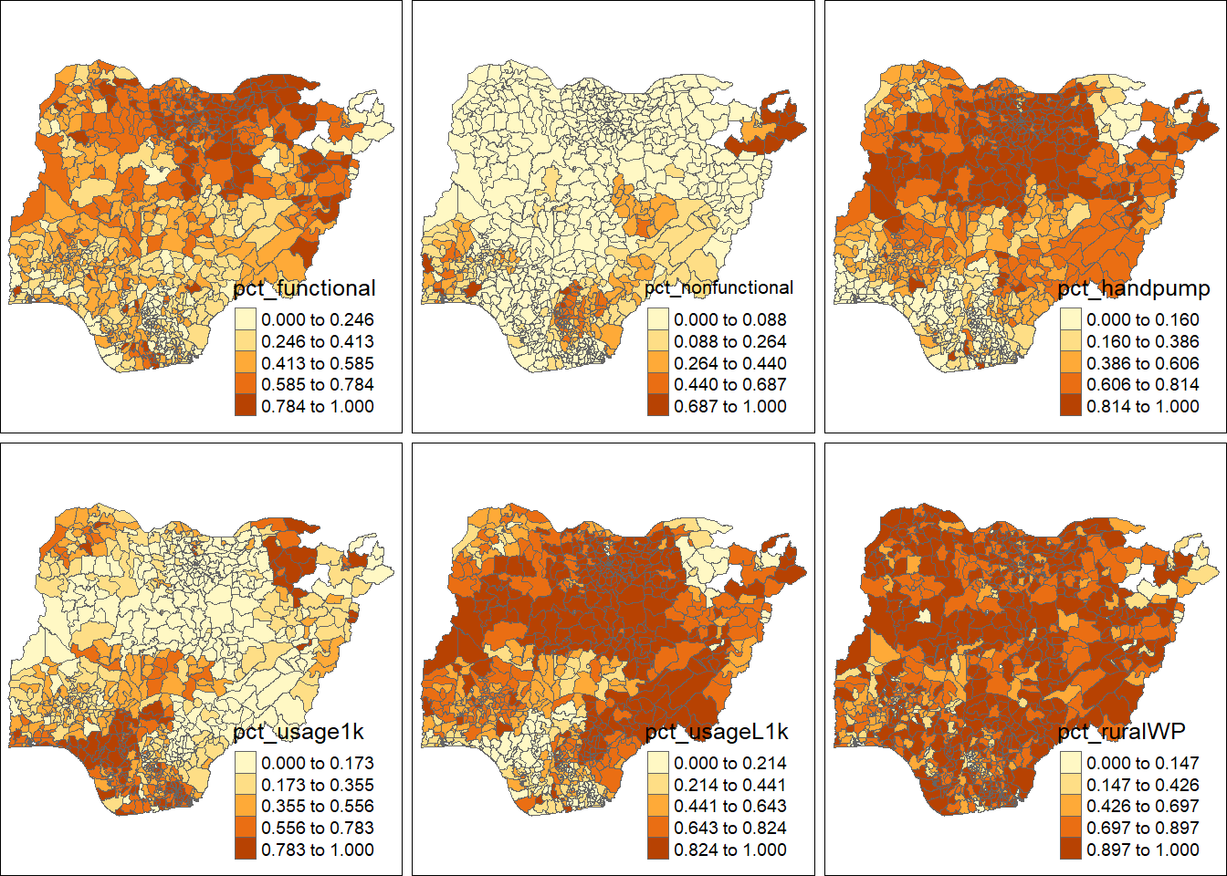
Correlation Analysis
Use corrplot() function of corrplot package to visualise and analyse the correlation of the input variables.
nga_sf_var <- nga_sf %>%
  st_drop_geometry() %>%
  select("shapeName", "functional","nonfunctional", "pct_functional", "pct_nonfunctional", "pct_handpump","pct_usage1k","pct_usageL1k", "pct_ruralWP")
cluster_vars.cor = cor(nga_sf_var[,2:8])
corrplot.mixed(cluster_vars.cor,
         lower = "ellipse",
               upper = "number",
               tl.pos = "lt",
               diag = "l",
               tl.col = "black")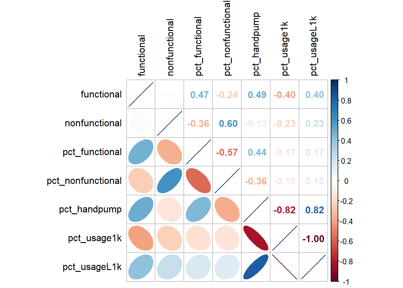
cluster_vars <- nga_sf_var %>%
  select("shapeName", "pct_functional", "pct_nonfunctional", "pct_handpump", "pct_usageL1k", "pct_ruralWP")
head(cluster_vars,10)
shapeName pct_functional pct_nonfunctional pct_handpump pct_usageL1k
1 aba north 0.4117647 0.05882353 0.11764706 0.17647059
2 aba south 0.4084507 0.09859155 0.09859155 0.12676056
4 abaji 0.4035088 0.00000000 0.40350877 0.40350877
5 abak 0.4791667 0.00000000 0.08333333 0.08333333
6 abakaliki 0.3519313 0.46781116 0.43776824 0.90557940
7 abeokuta north 0.4705882 0.08823529 0.14705882 0.23529412
8 abeokuta south 0.6050420 0.11764706 0.16806723 0.29411765
9 abi 0.5197368 0.07236842 0.59868421 0.67105263
10 aboh-mbaise 0.2727273 0.33333333 0.01515152 0.34848485
11 abua/odual 0.6410256 0.02564103 0.30769231 0.33333333
pct_ruralWP
1 0.00000000
2 0.05633803
4 0.84210526
5 0.83333333
6 0.87553648
7 0.20588235
8 0.00000000
9 0.95394737
10 0.72727273
11 0.53846154cluster_vars.cor = cor(cluster_vars[,2:6])
corrplot.mixed(cluster_vars.cor,
lower = "ellipse",
upper = "number",
tl.pos = "lt",
diag = "l",
tl.col = "black")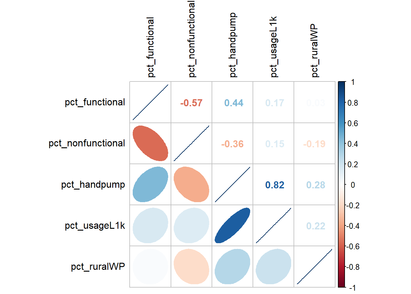
Hierarchy Cluster Analysis
Change the rows by town name instead of row number by using the code chunk below.
row.names(cluster_vars) <- cluster_vars$"shapeName"
head(cluster_vars,10)
shapeName pct_functional pct_nonfunctional pct_handpump
aba north aba north 0.4117647 0.05882353 0.11764706
aba south aba south 0.4084507 0.09859155 0.09859155
abaji abaji 0.4035088 0.00000000 0.40350877
abak abak 0.4791667 0.00000000 0.08333333
abakaliki abakaliki 0.3519313 0.46781116 0.43776824
abeokuta north abeokuta north 0.4705882 0.08823529 0.14705882
abeokuta south abeokuta south 0.6050420 0.11764706 0.16806723
abi abi 0.5197368 0.07236842 0.59868421
aboh-mbaise aboh-mbaise 0.2727273 0.33333333 0.01515152
abua/odual abua/odual 0.6410256 0.02564103 0.30769231
pct_usageL1k pct_ruralWP
aba north 0.17647059 0.00000000
aba south 0.12676056 0.05633803
abaji 0.40350877 0.84210526
abak 0.08333333 0.83333333
abakaliki 0.90557940 0.87553648
abeokuta north 0.23529412 0.20588235
abeokuta south 0.29411765 0.00000000
abi 0.67105263 0.95394737
aboh-mbaise 0.34848485 0.72727273
abua/odual 0.33333333 0.53846154Delete the shapeName field by using the code chunk below.
nga_cluster_var <- select(cluster_vars, c(2:6))
head(nga_cluster_var, 10)
pct_functional pct_nonfunctional pct_handpump pct_usageL1k
aba north 0.4117647 0.05882353 0.11764706 0.17647059
aba south 0.4084507 0.09859155 0.09859155 0.12676056
abaji 0.4035088 0.00000000 0.40350877 0.40350877
abak 0.4791667 0.00000000 0.08333333 0.08333333
abakaliki 0.3519313 0.46781116 0.43776824 0.90557940
abeokuta north 0.4705882 0.08823529 0.14705882 0.23529412
abeokuta south 0.6050420 0.11764706 0.16806723 0.29411765
abi 0.5197368 0.07236842 0.59868421 0.67105263
aboh-mbaise 0.2727273 0.33333333 0.01515152 0.34848485
abua/odual 0.6410256 0.02564103 0.30769231 0.33333333
pct_ruralWP
aba north 0.00000000
aba south 0.05633803
abaji 0.84210526
abak 0.83333333
abakaliki 0.87553648
abeokuta north 0.20588235
abeokuta south 0.00000000
abi 0.95394737
aboh-mbaise 0.72727273
abua/odual 0.53846154Min-Max standardisation
In the code chunk below, normalize() of heatmaply. package is used to stadardisation the clustering variables by using Min-Max method. The summary() is then used to display the summary statistics of the standardised clustering variables.
nga_cluster_var.std <- normalize(nga_cluster_var)
summary(nga_cluster_var.std)
pct_functional pct_nonfunctional pct_handpump pct_usageL1k
Min. :0.0000 Min. :0.0000 Min. :0.0000 Min. :0.0000
1st Qu.:0.3333 1st Qu.:0.0000 1st Qu.:0.1860 1st Qu.:0.4157
Median :0.4792 Median :0.0000 Median :0.5255 Median :0.6807
Mean :0.5070 Mean :0.1277 Mean :0.4956 Mean :0.6182
3rd Qu.:0.6749 3rd Qu.:0.2105 3rd Qu.:0.7857 3rd Qu.:0.8750
Max. :1.0000 Max. :1.0000 Max. :1.0000 Max. :1.0000
pct_ruralWP
Min. :0.0000
1st Qu.:0.5922
Median :0.8717
Mean :0.7395
3rd Qu.:1.0000
Max. :1.0000 Z-score standardisation
Z-score standardisation can be performed easily by using scale() of Base R. The code chunk below will be used to stadardisation the clustering variables by using Z-score method.
nga_cluster_var.z <- scale(nga_cluster_var)
describe(nga_cluster_var.z)
nga_cluster_var.z
5 Variables 761 Observations
--------------------------------------------------------------------------------
pct_functional
n missing distinct Info Mean Gmd .05 .10
761 0 619 1 4.388e-17 1.142 -1.4794 -1.2332
.25 .50 .75 .90 .95
-0.7384 -0.1182 0.7143 1.5062 1.7435
lowest : -2.155978 -2.082654 -2.027105 -1.919710 -1.872456
highest: 2.041621 2.055563 2.058539 2.079565 2.096853
--------------------------------------------------------------------------------
pct_nonfunctional
n missing distinct Info Mean Gmd .05
761 0 327 0.858 -2.745e-18 0.9202 -0.6244
.10 .25 .50 .75 .90 .95
-0.6244 -0.6244 -0.6244 0.4053 1.4028 2.0249
lowest : -0.6243907 -0.6007630 -0.5999768 -0.5983751 -0.5972189
highest: 3.5872460 3.6737018 3.6796302 3.8219119 4.2665422
--------------------------------------------------------------------------------
pct_handpump
n missing distinct Info Mean Gmd .05 .10
761 0 619 1 1.95e-17 1.151 -1.5333 -1.4366
.25 .50 .75 .90 .95
-0.9577 0.0927 0.8977 1.3315 1.4369
lowest : -1.533321 -1.505447 -1.503854 -1.493139 -1.492068
highest: 1.529392 1.532834 1.543799 1.543951 1.560645
--------------------------------------------------------------------------------
pct_usageL1k
n missing distinct Info Mean Gmd .05 .10
761 0 632 1 4.937e-17 1.126 -1.8933 -1.6260
.25 .50 .75 .90 .95
-0.6970 0.2150 0.8839 1.1195 1.2109
lowest : -2.127997 -2.096986 -2.079515 -2.075842 -2.064252
highest: 1.283139 1.283255 1.295455 1.295623 1.314196
--------------------------------------------------------------------------------
pct_ruralWP
n missing distinct Info Mean Gmd .05 .10
761 0 447 0.975 1.374e-16 1.038 -2.3488 -1.7713
.25 .50 .75 .90 .95
-0.4677 0.4200 0.8274 0.8274 0.8274
lowest : -2.3488119 -2.3224529 -2.3191273 -2.3160670 -2.3046972
highest: 0.8050784 0.8075325 0.8083123 0.8151828 0.8274464
--------------------------------------------------------------------------------Visualising the standardised clustering variables
The code chunk below plot the scaled pct_functional field.
r <- ggplot(data=nga_sf,
             aes(x= `pct_functional`)) +
  geom_histogram(bins=20,
                 color="black",
                 fill="light blue") +

  ggtitle("Raw values without standardisation")

nga_cluster_s_df <- as.data.frame(nga_cluster_var.std)
s <- ggplot(data=nga_cluster_s_df,
       aes(x=`pct_functional`)) +
  geom_histogram(bins=20,
                 color="black",
                 fill="light blue") +
  ggtitle("Min-Max Standardisation")

nga_cluster_z_df <- as.data.frame(nga_cluster_var.z)
z <- ggplot(data=nga_cluster_z_df,
       aes(x=`pct_functional`)) +
  geom_histogram(bins=20,
                 color="black",
                 fill="light blue") +
  ggtitle("Z-score Standardisation")

ggarrange(r, s, z,
          ncol = 3,
          nrow = 1)
r <- ggplot(data=nga_sf,
             aes(x= `pct_functional`)) +
  geom_density(color="black",
               fill="light blue") +
  ggtitle("Raw values without standardisation")

nga_cluster_s_df <- as.data.frame(nga_cluster_var.std)
s <- ggplot(data=nga_cluster_s_df,
       aes(x=`pct_functional`)) +
  geom_density(color="black",
               fill="light blue") +
  ggtitle("Min-Max Standardisation")

nga_cluster_z_df <- as.data.frame(nga_cluster_var.z)
z <- ggplot(data=nga_cluster_z_df,
       aes(x=`pct_functional`)) +
  geom_density(color="black",
               fill="light blue") +
  ggtitle("Z-score Standardisation")

ggarrange(r, s, z,
          ncol = 3,
          nrow = 1)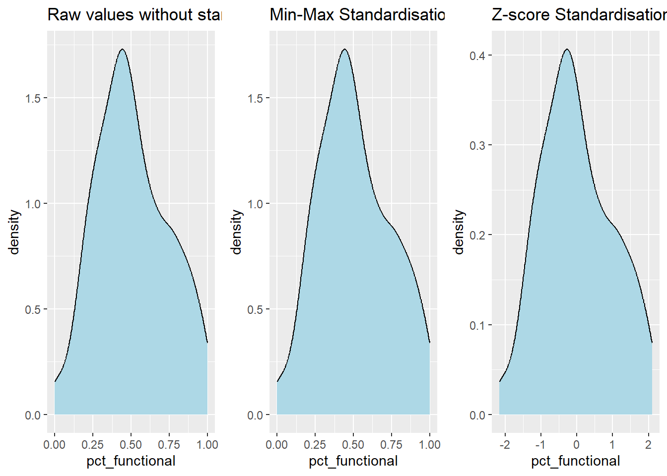
Computing proximity matrix
The code chunk below is used to compute the proximity matrix using euclidean method.
proxmat <- dist(nga_cluster_var, method = 'euclidean')Computing hierarchical clustering
The code chunk below performs hierarchical cluster analysis using ward.D method. The hierarchical clustering output is stored in an object of class hclust which describes the tree produced by the clustering process.
hclust_ward <- hclust(proxmat, method = 'ward.D')We can then plot the tree by using plot() of R Graphics as shown in the code chunk below.
plot(hclust_ward, cex = 0.6)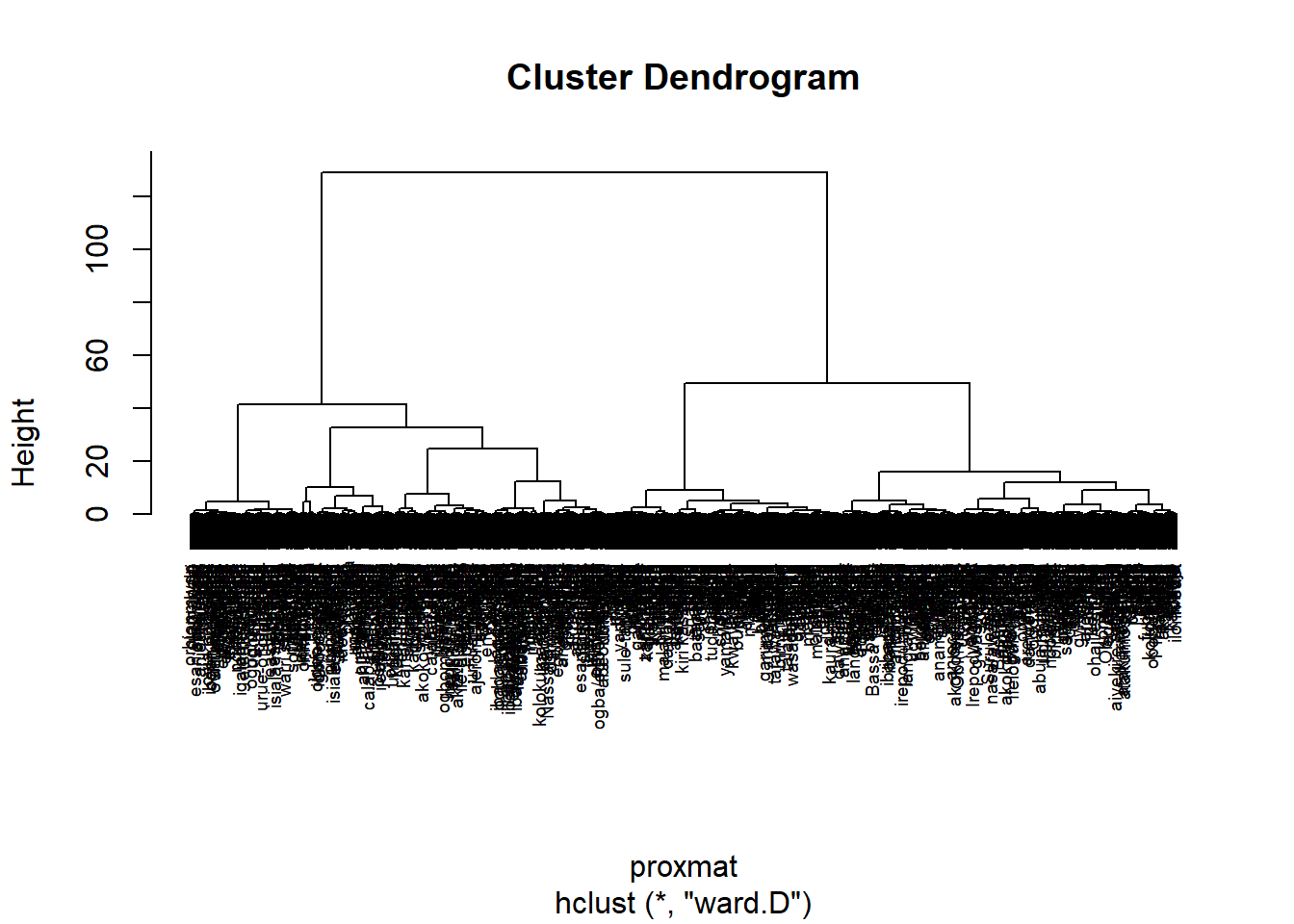
Selecting the optimal clustering algorithm
The code chunk below will be used to compute the agglomerative coefficients of all hierarchical clustering algorithms.
m <- c( "average", "single", "complete", "ward")
names(m) <- c( "average", "single", "complete", "ward")

ac <- function(x) {
  agnes(nga_cluster_var, method = x)$ac
}

map_dbl(m, ac)
average single complete ward
0.9320242 0.8841971 0.9557188 0.9930958 Determining Optimal Clusters
Another technical challenge face by data analyst in performing clustering analysis is to determine the optimal clusters to retain.
There are three commonly used methods to determine the optimal clusters, they are:
Elbow Method
Average Silhouette Method
Gap Statistic Method
Gap Statistic Method
The gap statistic compares the total within intra-cluster variation for different values of k with their expected values under null reference distribution of the data. The estimate of the optimal clusters will be value that maximize the gap statistic (i.e., that yields the largest gap statistic). This means that the clustering structure is far away from the random uniform distribution of points.
To compute the gap statistic, clusGap() of cluster package will be used.
set.seed(1234)
gap_stat <- clusGap(nga_cluster_var,
                    FUN = hcut,
                    nstart = 25,
                    K.max = 10,
                    B = 50)
# Print the result
print(gap_stat, method = "firstmax")
Clustering Gap statistic ["clusGap"] from call:
clusGap(x = nga_cluster_var, FUNcluster = hcut, K.max = 10, B = 50, nstart = 25)
B=50 simulated reference sets, k = 1..10; spaceH0="scaledPCA"
--> Number of clusters (method 'firstmax'): 5
logW E.logW gap SE.sim
[1,] 5.026463 5.468043 0.4415796 0.008773640
[2,] 4.784723 5.341867 0.5571439 0.013342806
[3,] 4.670536 5.257902 0.5873658 0.009107344
[4,] 4.588263 5.189318 0.6010551 0.009205690
[5,] 4.464084 5.136493 0.6724086 0.009032431
[6,] 4.420326 5.091754 0.6714280 0.008259398
[7,] 4.366689 5.051587 0.6848981 0.008286133
[8,] 4.333252 5.019084 0.6858326 0.008194347
[9,] 4.291669 4.993013 0.7013443 0.007706852
[10,] 4.251836 4.970142 0.7183058 0.007584662Visualise the plot by using fviz_gap_stat() of factoextra package.
fviz_gap_stat(gap_stat)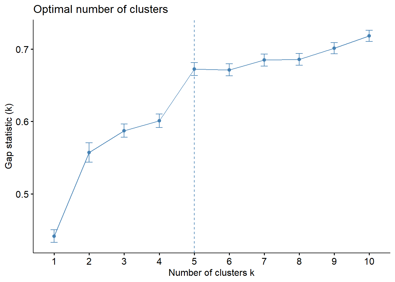
Interpreting the dendrograms
It’s also possible to draw the dendrogram with a border around the selected clusters by using rect.hclust() of R stats. The argument border is used to specify the border colors for the rectangles.
plot(hclust_ward, cex = 0.6)
rect.hclust(hclust_ward,
            k = 5,
            border = 2:5)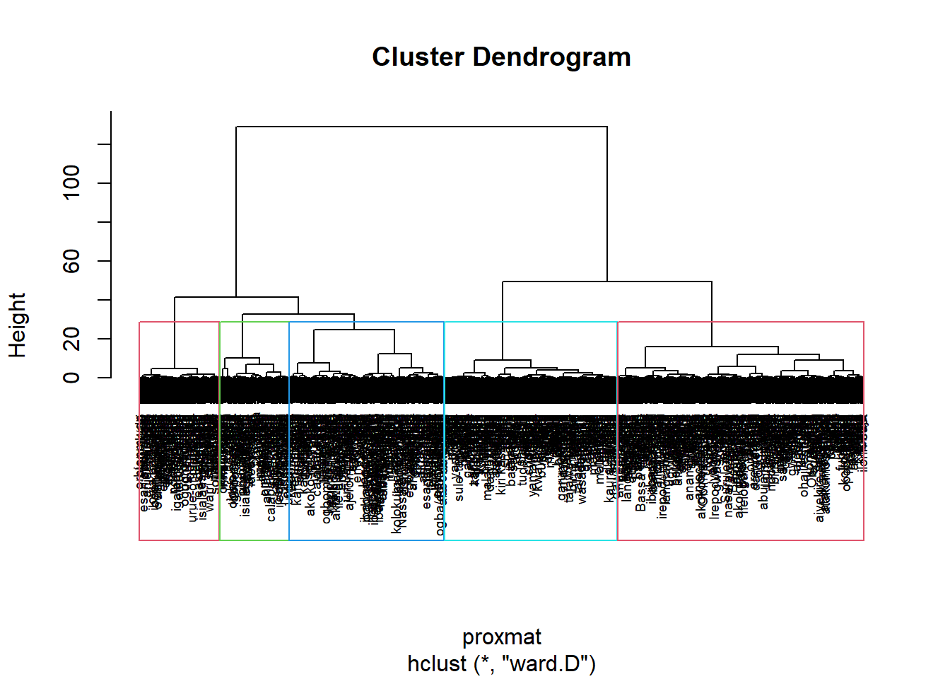
Visually-driven hierarchical clustering analysis
Transforming the data frame into a matrix
The code chunk below will be used to transform nga_cluster_var data frame into a data matrix.
nga_cluster_var_mat <- data.matrix(nga_cluster_var)Plotting interactive cluster heatmap using heatmaply()
In the code chunk below, the heatmaply() of heatmaply package is used to build an interactive cluster heatmap.
heatmaply(normalize(nga_cluster_var_mat),
          Colv=NA,
          dist_method = "euclidean",
          hclust_method = "ward.D",
          seriate = "OLO",
          colors = Blues,
          k_row = 5,
          margins = c(NA,200,60,NA),
          fontsize_row = 4,
          fontsize_col = 5,
          main="Geographic Segmentation of Nigeria WP indicators",
          xlab = "ICT Indicators",
          ylab = "ShapeName"
          )
Mapping the clusters formed
cutree() of R Base will be used in the code chunk below to derive a 5-cluster model.
groups <- as.factor(cutree(hclust_ward, k=5))The code chunk below form the join in three steps:
the groups list object will be converted into a matrix;
cbind() is used to append groups matrix onto shan_sf to produce an output simple feature object called
shan_sf_cluster; andrename of dplyr package is used to rename as.matrix.groups field as CLUSTER.
nga_sf_cluster <- cbind(nga_sf, as.matrix(groups)) %>%
  rename(`CLUSTER`=`as.matrix.groups.`)
qtm() of tmap package is used to plot the choropleth map showing the cluster formed.
qtm(nga_sf_cluster, "CLUSTER")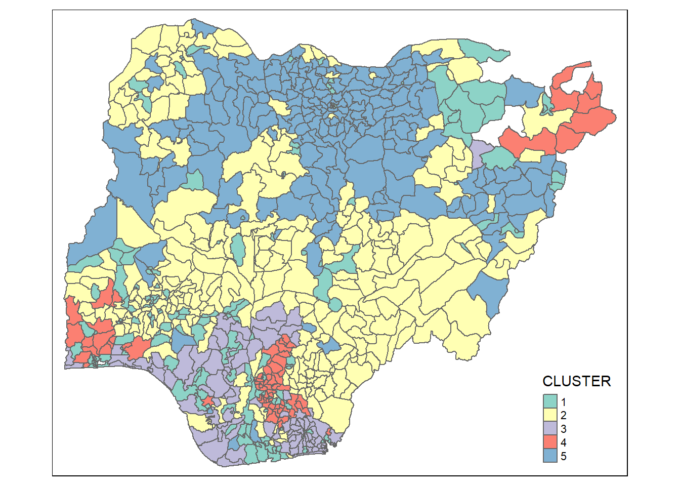
Converting into SpatialPolygonsDataFrame
The code chunk below uses as_Spatial() of sf package to convert nga_sf into a SpatialPolygonDataFrame called nga_sp.
nga_sp <- as_Spatial(nga_sf)nga.nb <- poly2nb(nga_sp, queen=TRUE)
summary(nga.nb)Neighbour list object:
Number of regions: 761
Number of nonzero links: 4348
Percentage nonzero weights: 0.750793
Average number of links: 5.713535
Link number distribution:
1 2 3 4 5 6 7 8 9 10 11 12 14
4 16 57 122 177 137 121 71 39 11 4 1 1
4 least connected regions:
138 509 525 560 with 1 link
1 most connected region:
508 with 14 linksComputing Neighbour List
poly2nd() of spdep package will be used to compute the neighbours list from polygon list.
nga.nb <- poly2nb(nga_sp, queen=TRUE)
summary(nga.nb)
Neighbour list object:
Number of regions: 761
Number of nonzero links: 4348
Percentage nonzero weights: 0.750793
Average number of links: 5.713535
Link number distribution:
1 2 3 4 5 6 7 8 9 10 11 12 14
4 16 57 122 177 137 121 71 39 11 4 1 1
4 least connected regions:
138 509 525 560 with 1 link
1 most connected region:
508 with 14 linksplot(nga_sp,
border=grey(.5))
plot(nga.nb,
coordinates(nga_sp),
col="blue",
add=TRUE)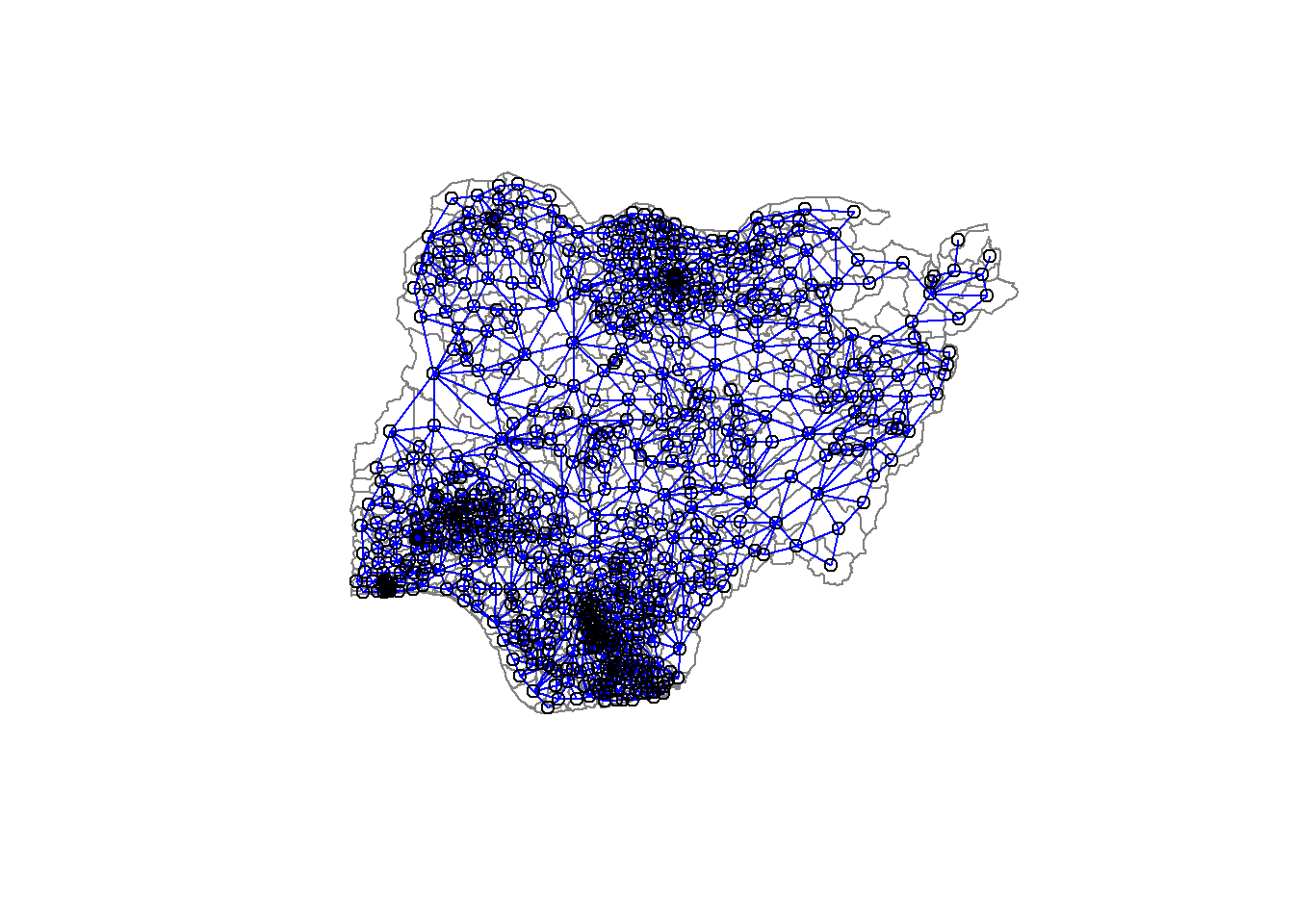
Computing minimum spanning tree
Calculating edge costs
The code chunk below is used to compute the cost of each edge.
lcosts <- nbcosts(nga.nb, nga_cluster_var)Note that we specify the style as B to make sure the cost values are not row-standardised.
nga.w <- nb2listw(nga.nb,
lcosts,
style="B")
summary(nga.w)Characteristics of weights list object:
Neighbour list object:
Number of regions: 761
Number of nonzero links: 4348
Percentage nonzero weights: 0.750793
Average number of links: 5.713535
Link number distribution:

  1   2   3   4   5   6   7   8   9  10  11  12  14
  4  16  57 122 177 137 121  71  39  11   4   1   1
4 least connected regions:
138 509 525 560 with 1 link
1 most connected region:
508 with 14 links
Weights style: B
Weights constants summary:
n nn S0 S1 S2
B 761 579121 1989.853 2574.866 26667.43Computing minimum spanning tree
The minimum spanning tree is computed by mean of the mstree(). of spdep package as shown in the code chunk below.
nga.mst <- mstree(nga.w)After computing the MST, we can check its class and dimension by using the code chunk below.
class(nga.mst)[1] "mst" "matrix"dim(nga.mst)[1] 760 3Display the content of nga.mst by using head() as shown in the code chunk below.
head(nga.mst) [,1] [,2] [,3]
[1,] 552 675 0.8654586
[2,] 675 650 0.4086729
[3,] 650 630 0.1229050
[4,] 650 749 0.1736307
[5,] 650 181 0.1923437
[6,] 650 365 0.2411888The plot method for the MST include a way to show the observation numbers of the nodes in addition to the edge. Plot this together with the town boundaries. We can see how the initial neighbour list is simplified to just one edge connecting each of the nodes, while passing through all the nodes.
plot(nga_sp, border=gray(.5))
plot.mst(nga.mst,
         coordinates(nga_sp),
         col="blue",
         cex.lab=0.7,
         cex.circles=0.005,
         add=TRUE)
Computing spatially constrained clusters using SKATER method
The code chunk below compute the spatially constrained cluster using skater() of spdep package.
clust5 <- spdep::skater(edges = nga.mst[,1:2],
                 data = nga_cluster_var,
                 method = "euclidean",
                 ncuts = 4)
The result of the skater() is an object of class skater. We can examine its contents by using the code chunk below.
str(clust5)List of 8
$ groups : num [1:761] 2 2 3 2 4 1 1 4 2 1 ...
$ edges.groups:List of 5
..$ :List of 3
.. ..$ node: num [1:161] 27 585 363 310 311 545 194 559 334 573 ...
.. ..$ edge: num [1:160, 1:3] 545 311 194 559 334 573 199 615 14 567 ...
.. ..$ ssw : num 85.1
..$ :List of 3
.. ..$ node: num [1:124] 33 102 65 101 332 717 539 214 9 359 ...
.. ..$ edge: num [1:123, 1:3] 9 359 538 214 539 717 332 101 65 102 ...
.. ..$ ssw : num 62.8
..$ :List of 3
.. ..$ node: num [1:193] 482 298 66 499 395 121 23 480 651 514 ...
.. ..$ edge: num [1:192, 1:3] 298 66 499 395 597 121 681 537 627 118 ...
.. ..$ ssw : num 81.4
..$ :List of 3
.. ..$ node: num [1:75] 234 723 443 161 711 461 413 722 408 727 ...
.. ..$ edge: num [1:74, 1:3] 13 564 533 408 455 215 491 401 281 408 ...
.. ..$ ssw : num 19.6
..$ :List of 3
.. ..$ node: num [1:208] 479 94 442 760 95 166 137 404 699 103 ...
.. ..$ edge: num [1:207, 1:3] 406 253 130 377 108 467 414 432 692 223 ...
.. ..$ ssw : num 87.1
$ not.prune : NULL
$ candidates : int [1:5] 1 2 3 4 5
$ ssto : num 441
$ ssw : num [1:5] 441 409 364 350 336
$ crit : num [1:2] 1 Inf
$ vec.crit : num [1:761] 1 1 1 1 1 1 1 1 1 1 ...
- attr(*, "class")= chr "skater"Check the cluster assignment by using the code chunk below.
ccs5 <- clust5$groups
ccs5
[1] 2 2 3 2 4 1 1 4 2 1 3 3 4 1 3 1 4 2 3 4 1 2 3 2 1 1 1 1 3 1 1 5 2 1 5 1 3
[38] 3 1 3 2 1 3 3 3 5 3 1 5 1 1 1 2 2 2 1 1 3 1 4 1 5 3 3 2 3 1 5 3 3 1 1 3 5
[75] 4 2 2 2 1 5 1 5 3 5 5 3 5 5 5 4 3 3 4 5 5 5 5 5 5 4 2 2 5 3 5 5 3 5 5 3 3
[112] 5 5 3 5 4 4 3 1 1 3 3 3 1 5 3 5 5 3 5 4 1 3 2 2 3 5 5 3 5 5 5 5 5 5 3 3 3
[149] 5 5 5 5 5 5 1 1 5 5 5 3 4 5 2 5 5 5 2 4 3 3 3 3 3 1 1 1 3 1 2 3 1 2 3 3 3
[186] 3 2 1 2 3 2 2 2 1 1 1 1 1 1 2 2 2 1 1 1 2 2 1 1 1 4 1 2 2 4 4 5 3 5 5 5 5
[223] 5 3 5 3 5 5 5 5 5 5 5 4 4 5 3 4 5 5 5 3 2 5 5 3 3 5 4 5 3 3 5 5 5 3 3 5 3
[260] 5 5 4 4 5 5 5 5 5 1 1 1 1 1 1 1 1 1 1 2 2 4 2 1 3 2 2 2 2 1 3 1 3 3 3 3 3
[297] 3 3 3 1 3 1 2 2 2 1 2 2 1 1 1 1 3 3 2 1 1 5 2 1 1 3 3 4 2 1 2 2 1 1 4 2 3
[334] 1 3 3 3 3 3 3 3 3 1 5 2 1 1 1 3 3 3 1 3 3 1 4 4 2 2 2 3 2 1 1 1 2 5 1 2 2
[371] 1 1 4 3 5 5 5 5 5 3 3 5 5 4 4 4 3 5 3 3 3 5 5 3 3 5 1 5 3 5 4 5 4 5 5 5 5
[408] 4 3 5 3 5 4 5 3 5 3 5 4 3 3 2 5 5 5 5 5 3 3 3 1 5 4 3 1 5 5 3 5 5 5 5 4 5
[445] 3 5 4 3 5 3 1 1 1 5 4 4 3 5 3 5 4 3 5 5 5 3 5 5 5 5 5 3 5 3 5 5 4 5 5 3 5
[482] 3 3 5 5 5 2 2 5 5 4 5 5 2 3 3 5 3 3 5 5 5 1 3 5 5 5 3 3 1 1 1 5 3 2 5 5 2
[519] 2 4 2 2 2 2 2 2 2 2 5 2 1 4 4 4 2 1 3 2 2 4 4 1 1 3 1 2 3 1 1 2 1 1 3 3 3
[556] 4 1 2 1 2 2 2 4 4 4 2 1 4 3 3 3 2 1 2 1 4 1 1 1 3 1 1 1 2 1 3 3 4 2 1 2 2
[593] 1 1 1 3 3 2 3 2 2 2 2 2 2 2 1 1 1 1 2 3 4 1 1 1 1 2 2 2 3 3 2 1 1 1 3 3 4
[630] 1 3 1 5 4 3 3 5 1 3 5 5 5 4 5 5 3 3 3 5 1 3 1 1 5 3 1 4 1 3 3 5 5 5 4 5 5
[667] 3 5 1 3 5 3 3 5 1 5 3 5 3 1 3 3 5 2 5 4 3 3 3 5 4 5 5 5 5 3 5 5 5 5 3 2 2
[704] 1 2 1 1 2 1 2 4 2 2 1 2 2 2 5 2 2 2 4 4 1 2 2 4 3 3 5 5 1 1 1 3 4 5 4 3 3
[741] 3 3 3 4 4 5 5 3 1 5 5 5 5 5 5 5 5 3 5 5 3table(ccs5)ccs5
1 2 3 4 5
161 124 193 75 208 Plot the pruned tree that shows the five clusters on top of the townshop area.
plot(nga_sp, border=gray(.5))
plot(clust5,
     coordinates(nga_sp),
     cex.lab=.7,
     groups.colors=c("red","green","blue", "brown", "pink"),
     cex.circles=0.005,
     add=TRUE)
Warning in segments(coords[id1, 1], coords[id1, 2], coords[id2, 1],
coords[id2, : "add" is not a graphical parameter
Warning in segments(coords[id1, 1], coords[id1, 2], coords[id2, 1],
coords[id2, : "add" is not a graphical parameter
Warning in segments(coords[id1, 1], coords[id1, 2], coords[id2, 1],
coords[id2, : "add" is not a graphical parameter
Warning in segments(coords[id1, 1], coords[id1, 2], coords[id2, 1],
coords[id2, : "add" is not a graphical parameter
Warning in segments(coords[id1, 1], coords[id1, 2], coords[id2, 1],
coords[id2, : "add" is not a graphical parameter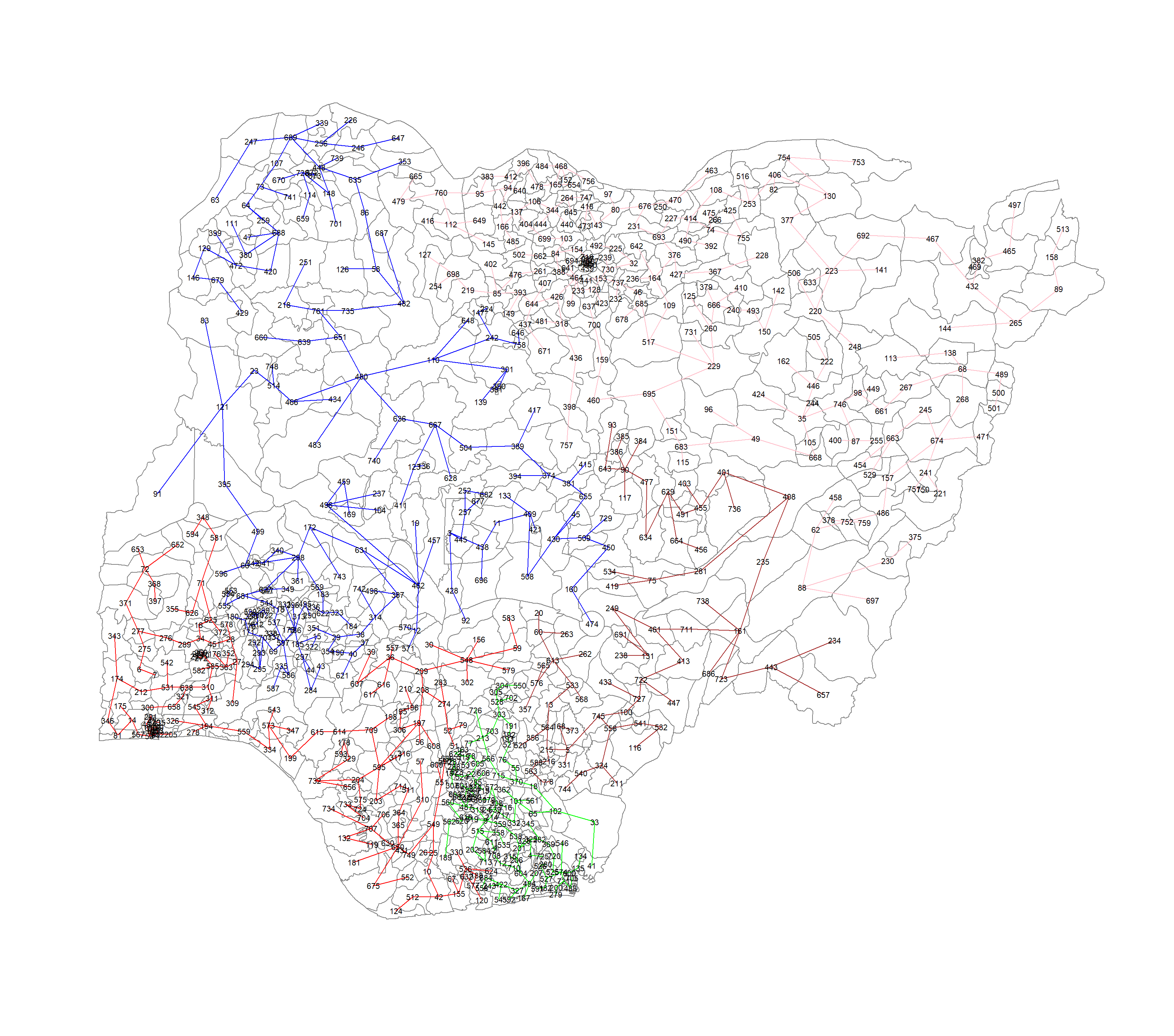
Visualising the clusters in choropleth map
The code chunk below is used to plot the newly derived clusters by using SKATER method.
groups_mat <- as.matrix(clust5$groups)
nga_sf_spatialcluster <- cbind(nga_sf_cluster, as.factor(groups_mat)) %>%
  rename(`SP_CLUSTER`=`as.factor.groups_mat.`)
qtm(nga_sf_spatialcluster, "SP_CLUSTER")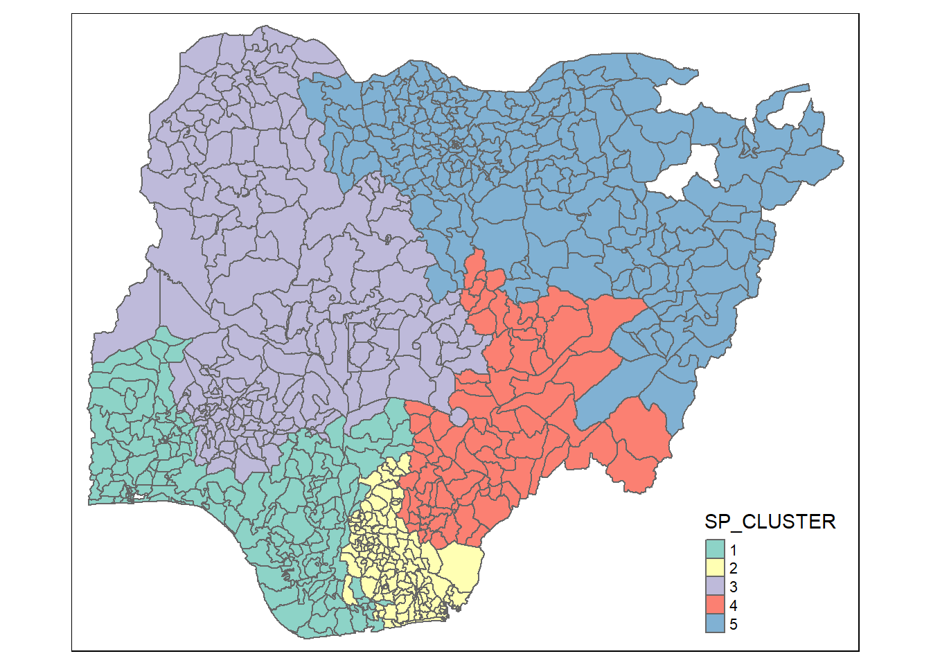
For easy comparison, it will be better to place both the hierarchical clustering and spatially constrained hierarchical clustering maps next to each other.
hclust.map <- qtm(nga_sf_cluster,
                  "CLUSTER", title = "Hierarchical clustering") +
  tm_borders(alpha = 0.5)

shclust.map <- qtm(nga_sf_spatialcluster,
                   "SP_CLUSTER", title = "spatially constrained clusters using SKATER method") +
  tm_borders(alpha = 0.5)

tmap_arrange(hclust.map, shclust.map,
             asp=NA, ncol=2)
Warning: One tm layer group has duplicated layer types, which are omitted. To
draw multiple layers of the same type, use multiple layer groups (i.e. specify
tm_shape prior to each of them).
Warning: One tm layer group has duplicated layer types, which are omitted. To
draw multiple layers of the same type, use multiple layer groups (i.e. specify
tm_shape prior to each of them).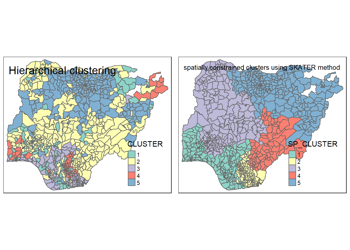
Spatially Constrained Clustering: ClustGeo Method
Ward-like hierarchical clustering: ClustGeo
To perform non-spatially constrained hierarchical clustering, we only need to provide the function a dissimilarity matrix as shown in the code chunk below.
nongeo_cluster <- hclustgeo(proxmat)
plot(nongeo_cluster, cex = 0.5)
rect.hclust(nongeo_cluster,
            k = 5,
            border = 2:5)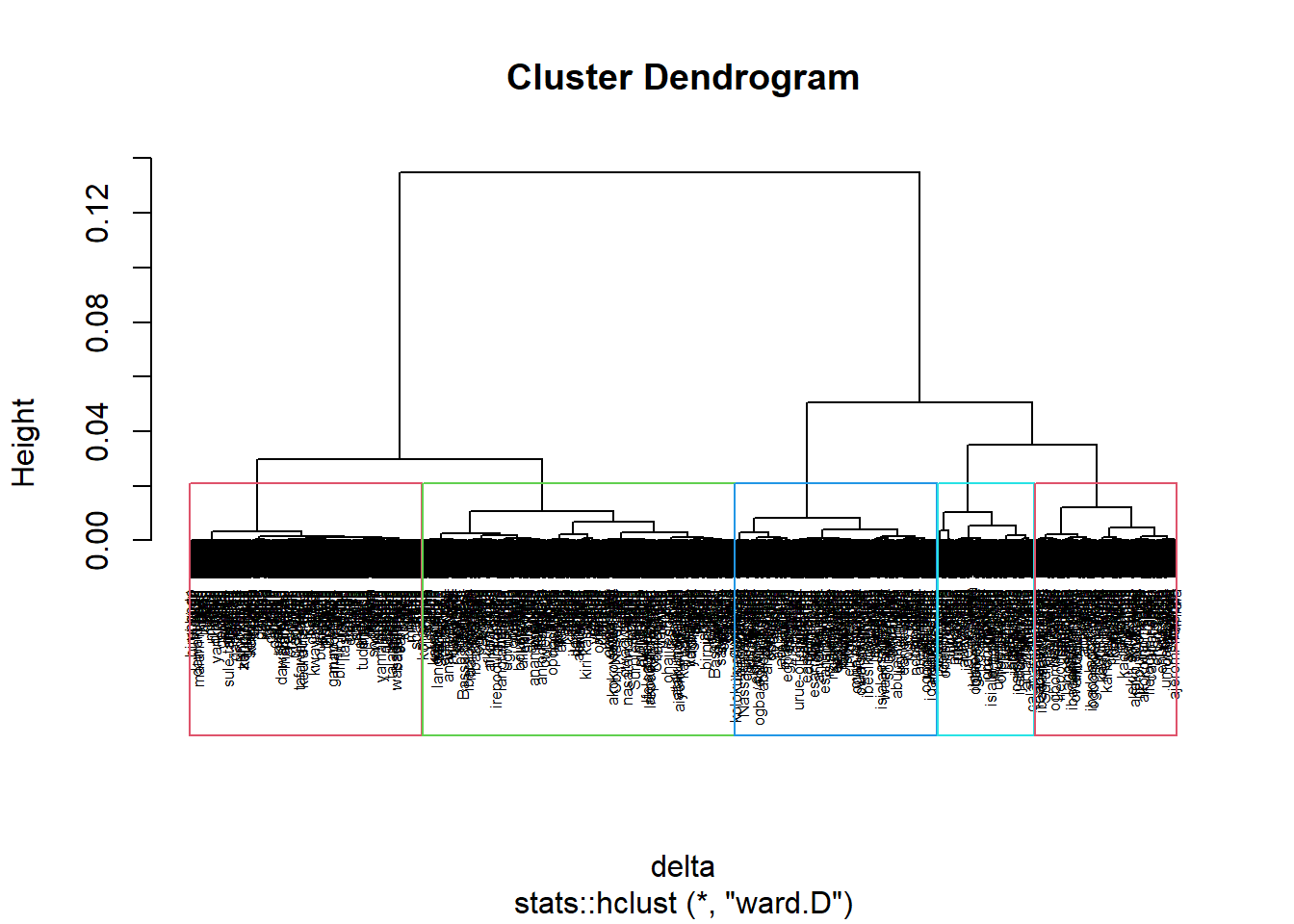
Mapping the clusters formed
Plot the clusters on a categorical area shaded map by using code chunk below.
groups <- as.factor(cutree(nongeo_cluster, k=5))nga_sf_ngeo_cluster <- cbind(nga_sf, as.matrix(groups)) %>%
rename(`CLUSTER` = `as.matrix.groups.`)qtm(nga_sf_ngeo_cluster, "CLUSTER")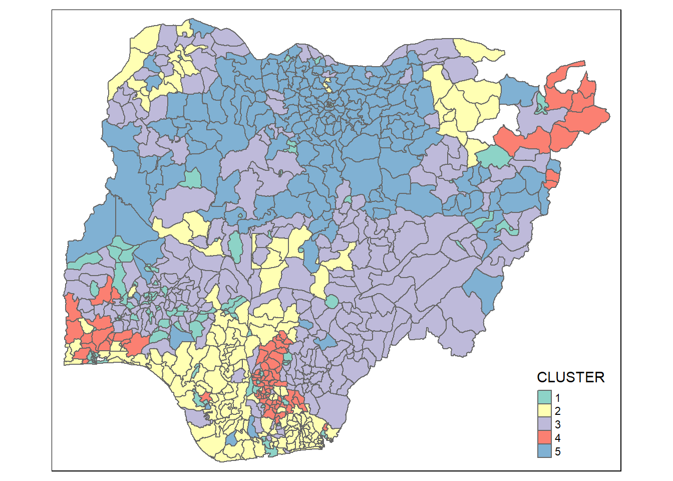
Spatially Constrained Hierarchical Clustering
Aspatial distance matrix will be derived by using st_distance() of sf package.
dist <- st_distance(nga_sf, nga_sf)
distmat <- as.dist(dist)
choicealpha() will be used to determine a suitable value for the mixing parameter alpha as shown in the code chunk below.
cr <- choicealpha(proxmat, distmat, range.alpha = seq(0, 1, 0.1), K=5, graph = TRUE)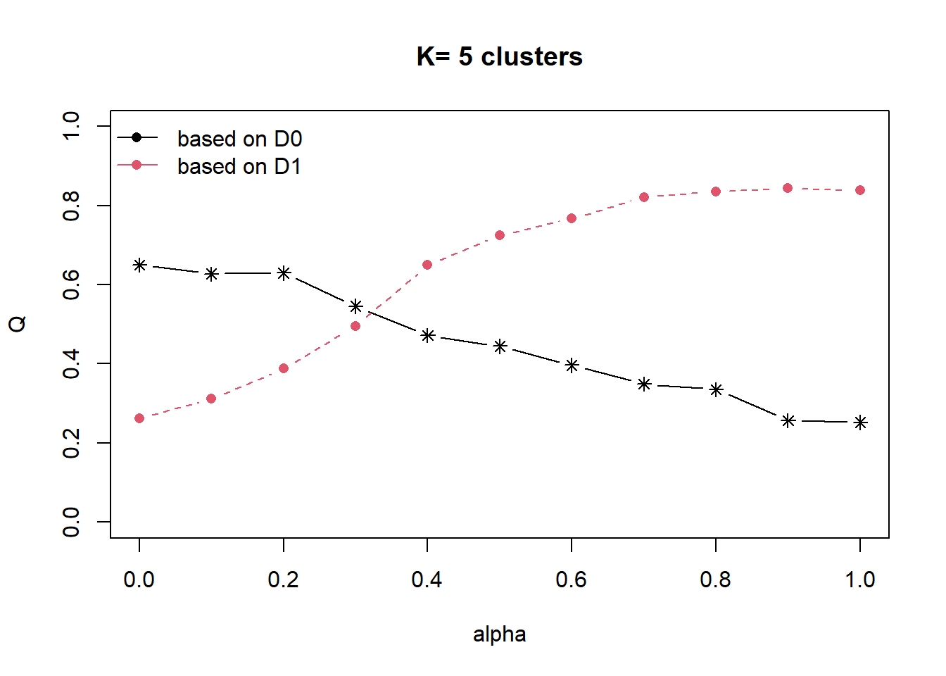
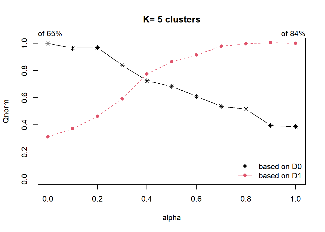
With reference to the graphs above, alpha = 0.4 will be used as shown in the code chunk below.
clustG <- hclustgeo(proxmat, distmat, alpha = 0.4)cutree() is used to derive the cluster objecct.
groups <- as.factor(cutree(clustG, k=5))Join back the group list with nga_sf polygon feature data frame by using the code chunk below.
nga_sf_Gcluster <- cbind(nga_sf, as.matrix(groups)) %>%
  rename(`CLUSTER` = `as.matrix.groups.`)
Plot the map of the newly delineated spatially constrained clusters.
qtm(nga_sf_Gcluster, "CLUSTER")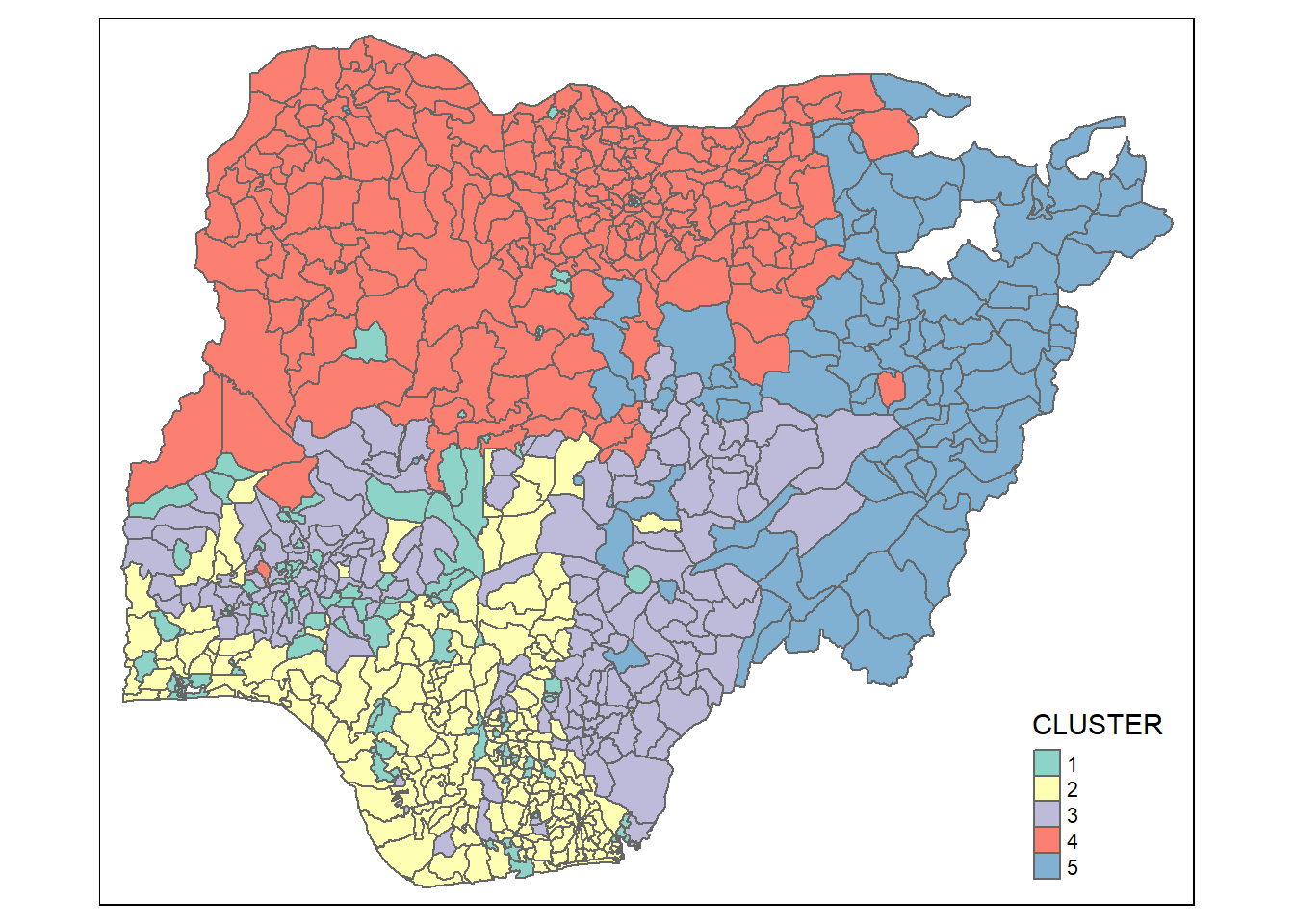
Visual Interpretation of Clusters
Multivariate Visualisation
Past studies shown that parallel coordinate plot can be used to reveal clustering variables by cluster very effectively. In the code chunk below, ggparcoord() of GGally package
ggparcoord(data = nga_sf_Gcluster,
           columns = c(10:15),
           groupColumn = "CLUSTER",
           scale = "std",
           alphaLines = 0.2,
           boxplot = TRUE,
           title = "Multiple Parallel Coordinates Plots of Nigeria Variables by Cluster") +
  facet_grid(~ CLUSTER) +
theme(axis.text.x = element_text(angle = 30, size = 15)) 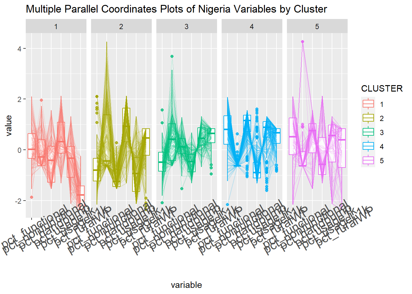
In the code chunk below, group_by() and summarise() of dplyr are used to derive mean values of the clustering variables.
nga_sf_Gcluster %>%
  st_set_geometry(NULL) %>%
  group_by(CLUSTER) %>%
  summarise(mean_pct_functional = mean(pct_functional),
            mean_pct_nonfunctional = mean(pct_nonfunctional),
            mean_pct_handpump = mean(pct_handpump),
            mean_pct_usage1k = mean(pct_usage1k),
            mean_pct_usageL1k = mean(pct_usageL1k),
            mean_pct_ruralWP = mean(pct_ruralWP))
# A tibble: 5 × 7
CLUSTER mean_pct_functional mean_pct_nonfunc…¹ mean_…² mean_…³ mean_…⁴ mean_…⁵
<chr> <dbl> <dbl> <dbl> <dbl> <dbl> <dbl>
1 1 0.540 0.117 0.363 0.509 0.491 0.191
2 2 0.344 0.200 0.147 0.643 0.357 0.803
3 3 0.391 0.216 0.542 0.242 0.758 0.893
4 4 0.683 0.00508 0.807 0.184 0.816 0.892
5 5 0.603 0.117 0.622 0.344 0.656 0.713
# … with abbreviated variable names ¹mean_pct_nonfunctional,
# ²mean_pct_handpump, ³mean_pct_usage1k, ⁴mean_pct_usageL1k,
# ⁵mean_pct_ruralWP