In-class Exercise 1

Overview

In this hands-on exercise, you will learn how to compute spatial weights using R. By the end to this hands-on exercise, you will be able to:

• import geospatial data using appropriate function(s) of sf package,

• import csv file using appropriate function of readr package,

• perform relational join using appropriate join function of dplyr package,

• compute spatial weights using appropriate functions of spdep package, and

• calculate spatially lagged variables using appropriate functions of spdep package.

Getting Started

The code chunk below will install an load spdep, tmap, tidyverse and sf packages.

pacman::p_load(sf,tidyverse,spdep,tmap)

Getting the Data Into R Environment

Importing Geospatial Data.

Importing polygon features

This code chunk will import ESRI shapefile into R.

hunan <- st_read(dsn = "data/geospatial", 
                layer = "Hunan")

Reading layer `Hunan' from data source 
  `D:\yuetongz\ISSS624\In-class_Ex\In-class_Ex1\data\geospatial' 
  using driver `ESRI Shapefile'
Simple feature collection with 88 features and 7 fields
Geometry type: POLYGON
Dimension:     XY
Bounding box:  xmin: 108.7831 ymin: 24.6342 xmax: 114.2544 ymax: 30.12812
Geodetic CRS:  WGS 84

Importing attribute data in csv

hunan2012 <- read_csv("data/aspatial/Hunan_2012.csv")

Rows: 88 Columns: 29
── Column specification ────────────────────────────────────────────────────────
Delimiter: ","
chr  (2): County, City
dbl (27): avg_wage, deposite, FAI, Gov_Rev, Gov_Exp, GDP, GDPPC, GIO, Loan, ...

ℹ Use `spec()` to retrieve the full column specification for this data.
ℹ Specify the column types or set `show_col_types = FALSE` to quiet this message.

Performing relational join

hunan <- left_join(hunan,hunan2012)

Joining, by = "County"

Visualising Regional Development Indicator

basemap <- tm_shape(hunan) +
  tm_polygons() +
  tm_text("NAME_3", size=0.5)

gdppc <- qtm(hunan, "GDPPC")
tmap_arrange(basemap, gdppc, asp=1, ncol=2)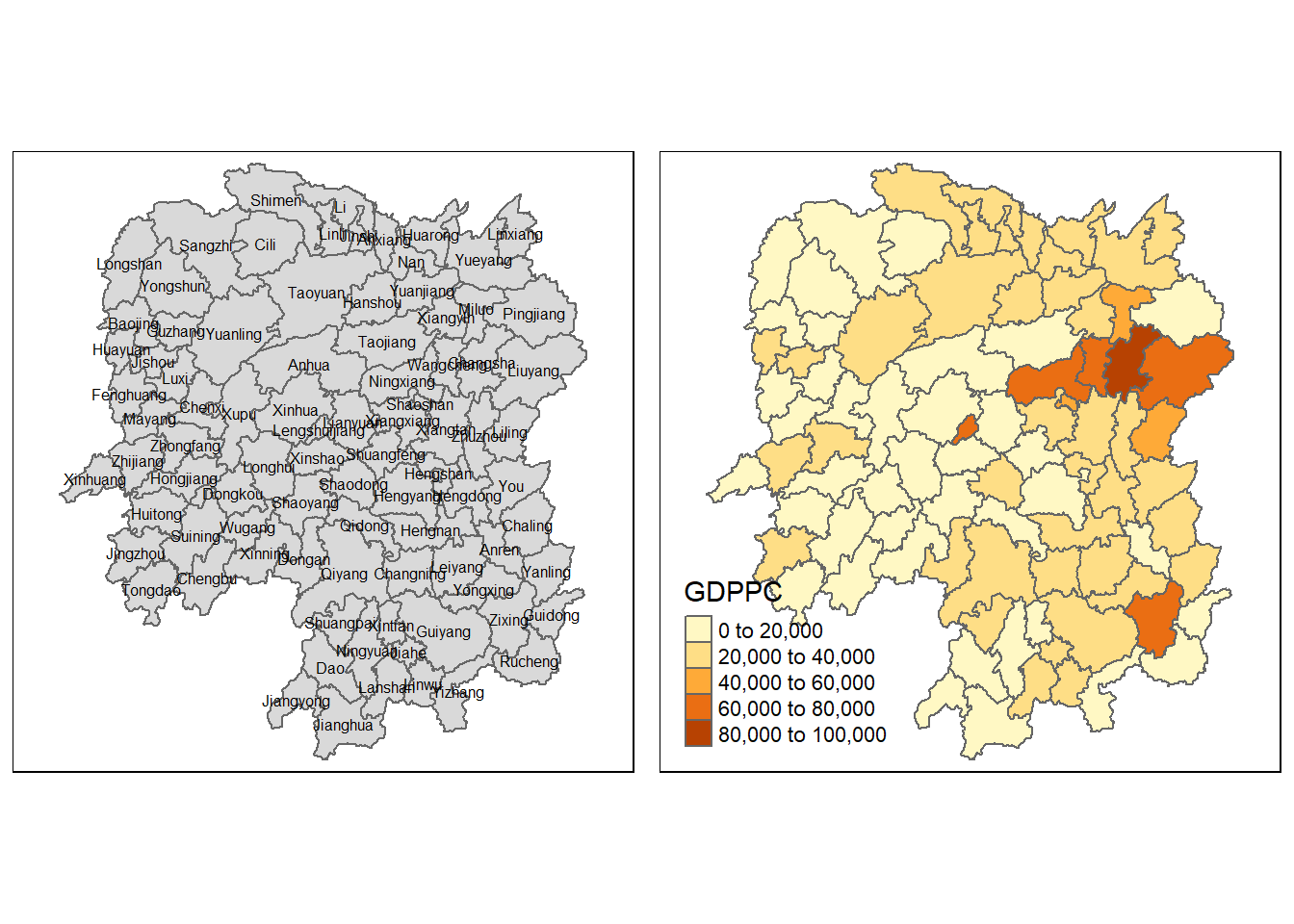

Computing Contiguity Spatial Weights

Computing(QUEEN) contiguity weight matrix

wm_q <- poly2nb(hunan, queen=TRUE)
summary(wm_q)

Neighbour list object:
Number of regions: 88 
Number of nonzero links: 448 
Percentage nonzero weights: 5.785124 
Average number of links: 5.090909 
Link number distribution:

 1  2  3  4  5  6  7  8  9 11 
 2  2 12 16 24 14 11  4  2  1 
2 least connected regions:
30 65 with 1 link
1 most connected region:
85 with 11 links

wm_q[[1]]

[1]  2  3  4 57 85

hunan$County[1]

[1] "Anxiang"

hunan$NAME_3[c(2,3,4,57,85)]

[1] "Hanshou" "Jinshi"  "Li"      "Nan"     "Taoyuan"

nb1 <- wm_q[[1]]
nb1 <- hunan$GDPPC[nb1]
nb1

[1] 20981 34592 24473 21311 22879

str(wm_q)

List of 88
 $ : int [1:5] 2 3 4 57 85
 $ : int [1:5] 1 57 58 78 85
 $ : int [1:4] 1 4 5 85
 $ : int [1:4] 1 3 5 6
 $ : int [1:4] 3 4 6 85
 $ : int [1:5] 4 5 69 75 85
 $ : int [1:4] 67 71 74 84
 $ : int [1:7] 9 46 47 56 78 80 86
 $ : int [1:6] 8 66 68 78 84 86
 $ : int [1:8] 16 17 19 20 22 70 72 73
 $ : int [1:3] 14 17 72
 $ : int [1:5] 13 60 61 63 83
 $ : int [1:4] 12 15 60 83
 $ : int [1:3] 11 15 17
 $ : int [1:4] 13 14 17 83
 $ : int [1:5] 10 17 22 72 83
 $ : int [1:7] 10 11 14 15 16 72 83
 $ : int [1:5] 20 22 23 77 83
 $ : int [1:6] 10 20 21 73 74 86
 $ : int [1:7] 10 18 19 21 22 23 82
 $ : int [1:5] 19 20 35 82 86
 $ : int [1:5] 10 16 18 20 83
 $ : int [1:7] 18 20 38 41 77 79 82
 $ : int [1:5] 25 28 31 32 54
 $ : int [1:5] 24 28 31 33 81
 $ : int [1:4] 27 33 42 81
 $ : int [1:3] 26 29 42
 $ : int [1:5] 24 25 33 49 54
 $ : int [1:3] 27 37 42
 $ : int 33
 $ : int [1:8] 24 25 32 36 39 40 56 81
 $ : int [1:8] 24 31 50 54 55 56 75 85
 $ : int [1:5] 25 26 28 30 81
 $ : int [1:3] 36 45 80
 $ : int [1:6] 21 41 47 80 82 86
 $ : int [1:6] 31 34 40 45 56 80
 $ : int [1:4] 29 42 43 44
 $ : int [1:4] 23 44 77 79
 $ : int [1:5] 31 40 42 43 81
 $ : int [1:6] 31 36 39 43 45 79
 $ : int [1:6] 23 35 45 79 80 82
 $ : int [1:7] 26 27 29 37 39 43 81
 $ : int [1:6] 37 39 40 42 44 79
 $ : int [1:4] 37 38 43 79
 $ : int [1:6] 34 36 40 41 79 80
 $ : int [1:3] 8 47 86
 $ : int [1:5] 8 35 46 80 86
 $ : int [1:5] 50 51 52 53 55
 $ : int [1:4] 28 51 52 54
 $ : int [1:5] 32 48 52 54 55
 $ : int [1:3] 48 49 52
 $ : int [1:5] 48 49 50 51 54
 $ : int [1:3] 48 55 75
 $ : int [1:6] 24 28 32 49 50 52
 $ : int [1:5] 32 48 50 53 75
 $ : int [1:7] 8 31 32 36 78 80 85
 $ : int [1:6] 1 2 58 64 76 85
 $ : int [1:5] 2 57 68 76 78
 $ : int [1:4] 60 61 87 88
 $ : int [1:4] 12 13 59 61
 $ : int [1:7] 12 59 60 62 63 77 87
 $ : int [1:3] 61 77 87
 $ : int [1:4] 12 61 77 83
 $ : int [1:2] 57 76
 $ : int 76
 $ : int [1:5] 9 67 68 76 84
 $ : int [1:4] 7 66 76 84
 $ : int [1:5] 9 58 66 76 78
 $ : int [1:3] 6 75 85
 $ : int [1:3] 10 72 73
 $ : int [1:3] 7 73 74
 $ : int [1:5] 10 11 16 17 70
 $ : int [1:5] 10 19 70 71 74
 $ : int [1:6] 7 19 71 73 84 86
 $ : int [1:6] 6 32 53 55 69 85
 $ : int [1:7] 57 58 64 65 66 67 68
 $ : int [1:7] 18 23 38 61 62 63 83
 $ : int [1:7] 2 8 9 56 58 68 85
 $ : int [1:7] 23 38 40 41 43 44 45
 $ : int [1:8] 8 34 35 36 41 45 47 56
 $ : int [1:6] 25 26 31 33 39 42
 $ : int [1:5] 20 21 23 35 41
 $ : int [1:9] 12 13 15 16 17 18 22 63 77
 $ : int [1:6] 7 9 66 67 74 86
 $ : int [1:11] 1 2 3 5 6 32 56 57 69 75 ...
 $ : int [1:9] 8 9 19 21 35 46 47 74 84
 $ : int [1:4] 59 61 62 88
 $ : int [1:2] 59 87
 - attr(*, "class")= chr "nb"
 - attr(*, "region.id")= chr [1:88] "1" "2" "3" "4" ...
 - attr(*, "call")= language poly2nb(pl = hunan, queen = TRUE)
 - attr(*, "type")= chr "queen"
 - attr(*, "sym")= logi TRUE

Creating(ROOK) contiguity based neighbours

wm_r <- poly2nb(hunan, queen=FALSE)
summary(wm_r)

Neighbour list object:
Number of regions: 88 
Number of nonzero links: 440 
Percentage nonzero weights: 5.681818 
Average number of links: 5 
Link number distribution:

 1  2  3  4  5  6  7  8  9 10 
 2  2 12 20 21 14 11  3  2  1 
2 least connected regions:
30 65 with 1 link
1 most connected region:
85 with 10 links

Visualising contiguity weights

longitude <- map_dbl(hunan$geometry, ~st_centroid(.x)[[1]])

latitude <- map_dbl(hunan$geometry, ~st_centroid(.x)[[2]])

Combine longitude and latitude

coords <- cbind(longitude, latitude)

head(coords)

     longitude latitude
[1,]  112.1531 29.44362
[2,]  112.0372 28.86489
[3,]  111.8917 29.47107
[4,]  111.7031 29.74499
[5,]  111.6138 29.49258
[6,]  111.0341 29.79863

Plotting Queen contiguity based neighbours map

plot(hunan$geometry, border="lightgrey")
plot(wm_q, coords, pch = 19, cex = 0.6, add = TRUE, col= "red")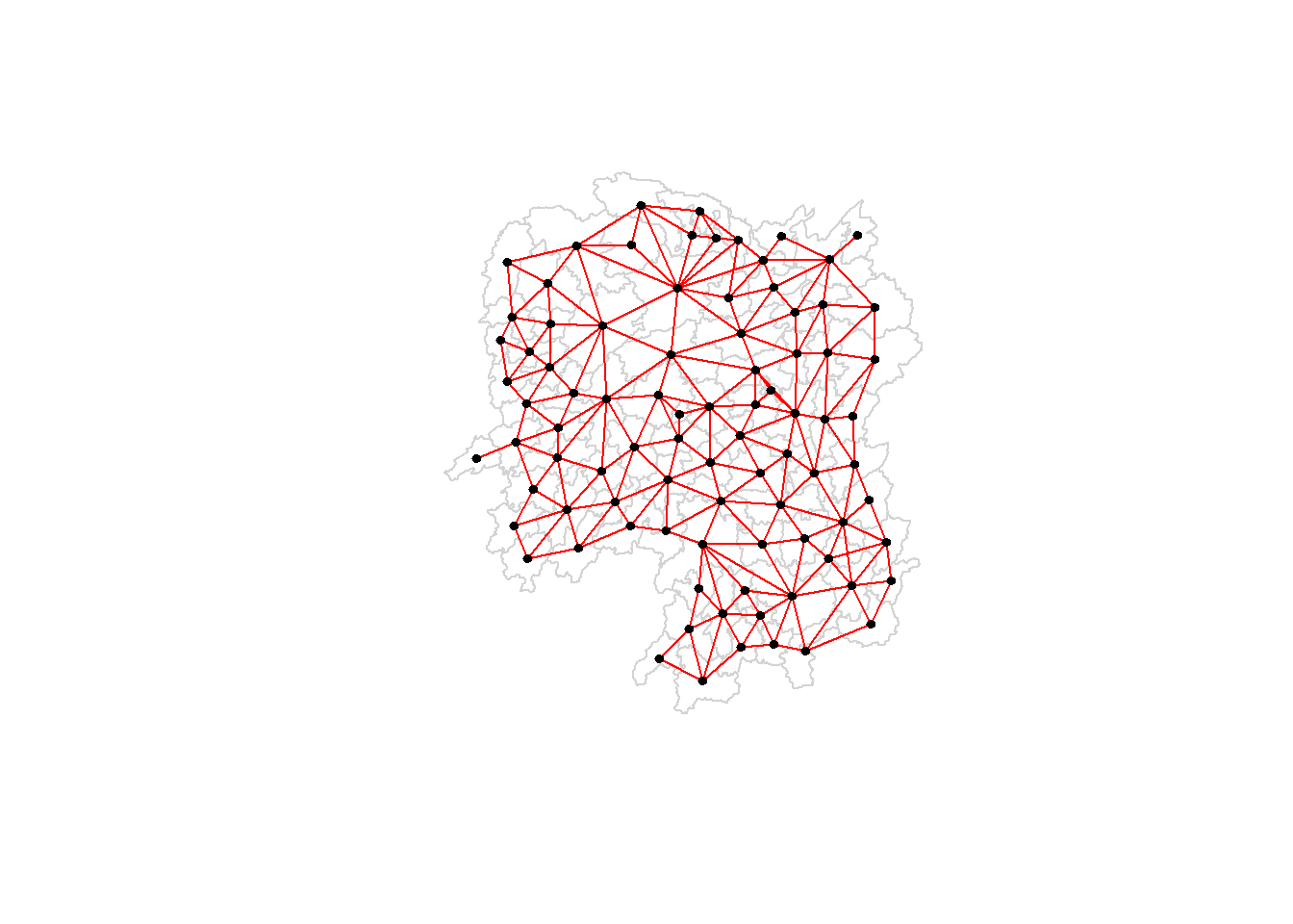

Plotting Rook contiguity based neighbours map

plot(hunan$geometry, border="lightgrey")
plot(wm_r, coords, pch = 19, cex = 0.6, add = TRUE, col = "red")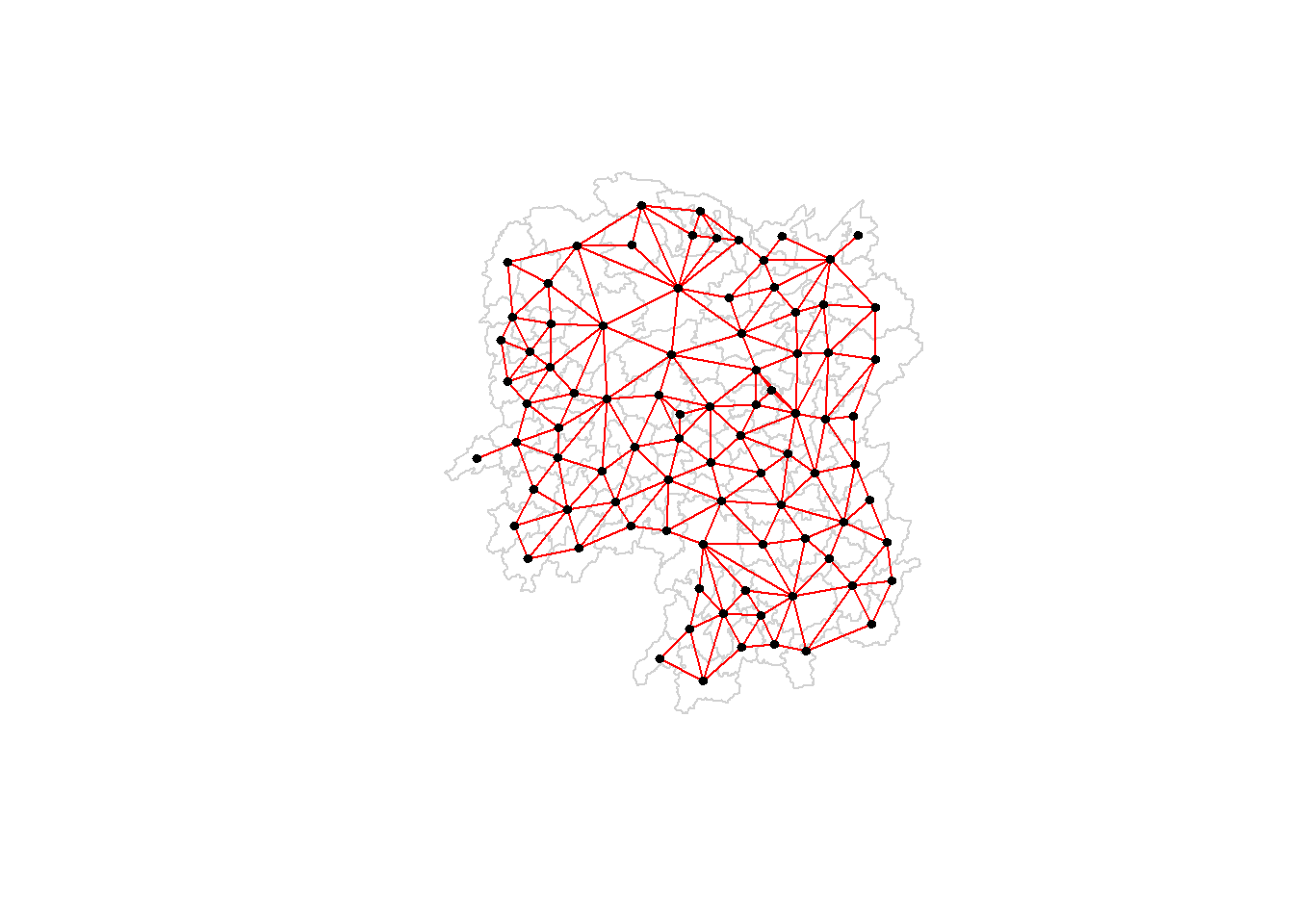

Plotting both Queen and Rook contiguity based neighbours maps

par(mfrow=c(1,2))
plot(hunan$geometry, border="lightgrey")
plot(wm_q, coords, pch = 19, cex = 0.6, add = TRUE, col= "red", main="Queen Contiguity")
plot(hunan$geometry, border="lightgrey")
plot(wm_r, coords, pch = 19, cex = 0.6, add = TRUE, col = "red", main="Rook Contiguity")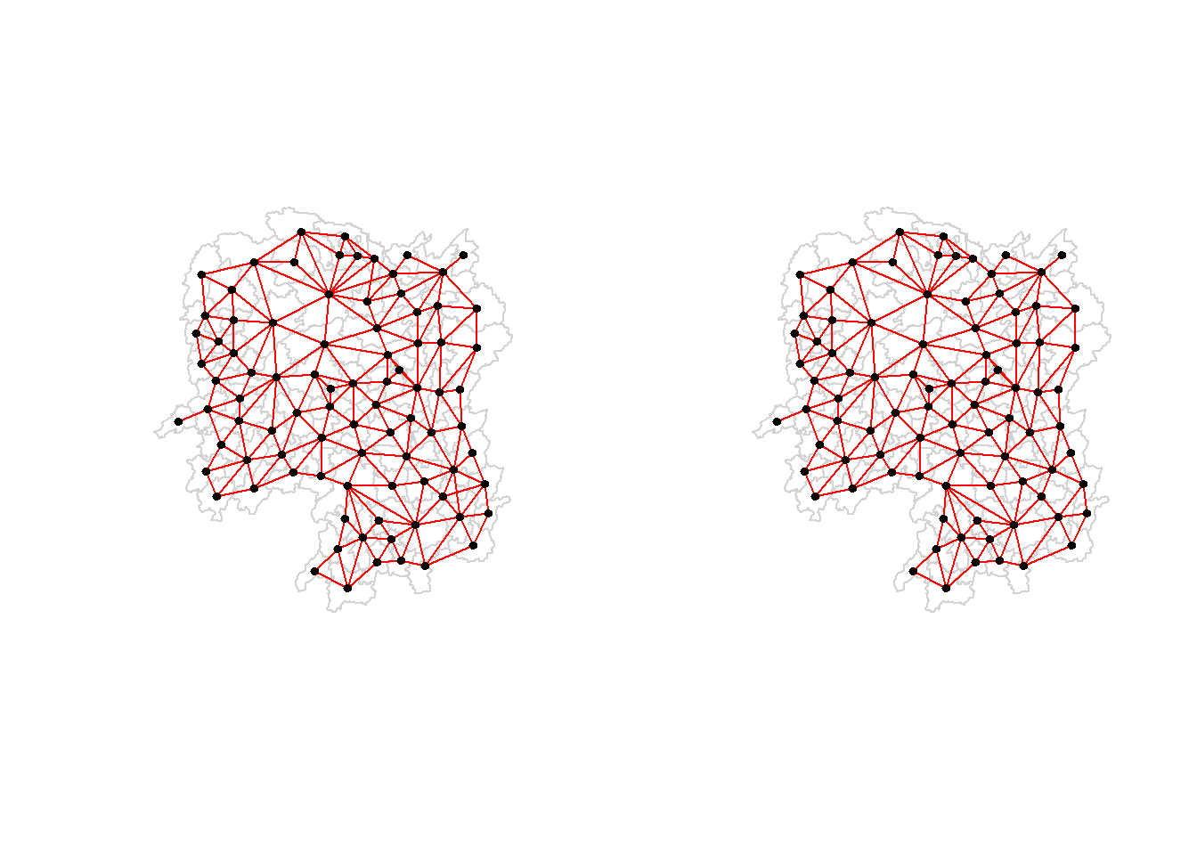

Computing distance based neighbours

Determine the cut-off distance

#coords <- coordinates(hunan)
k1 <- knn2nb(knearneigh(coords))
k1dists <- unlist(nbdists(k1, coords, longlat = TRUE))
summary(k1dists)

   Min. 1st Qu.  Median    Mean 3rd Qu.    Max. 
  24.79   32.57   38.01   39.07   44.52   61.79 

Computing fixed distance weight matrix

wm_d62 <- dnearneigh(coords, 0, 62, longlat = TRUE)
wm_d62

Neighbour list object:
Number of regions: 88 
Number of nonzero links: 324 
Percentage nonzero weights: 4.183884 
Average number of links: 3.681818 

Quiz: What is the meaning of “Average number of links: 3.681818” shown above?

Answer: On average, each area has 3.681818 neighbors.

Display wm_d62

str(wm_d62)

List of 88
 $ : int [1:5] 3 4 5 57 64
 $ : int [1:4] 57 58 78 85
 $ : int [1:4] 1 4 5 57
 $ : int [1:3] 1 3 5
 $ : int [1:4] 1 3 4 85
 $ : int 69
 $ : int [1:2] 67 84
 $ : int [1:4] 9 46 47 78
 $ : int [1:4] 8 46 68 84
 $ : int [1:4] 16 22 70 72
 $ : int [1:3] 14 17 72
 $ : int [1:5] 13 60 61 63 83
 $ : int [1:4] 12 15 60 83
 $ : int [1:2] 11 17
 $ : int 13
 $ : int [1:4] 10 17 22 83
 $ : int [1:3] 11 14 16
 $ : int [1:3] 20 22 63
 $ : int [1:5] 20 21 73 74 82
 $ : int [1:5] 18 19 21 22 82
 $ : int [1:6] 19 20 35 74 82 86
 $ : int [1:4] 10 16 18 20
 $ : int [1:3] 41 77 82
 $ : int [1:4] 25 28 31 54
 $ : int [1:4] 24 28 33 81
 $ : int [1:4] 27 33 42 81
 $ : int [1:2] 26 29
 $ : int [1:6] 24 25 33 49 52 54
 $ : int [1:2] 27 37
 $ : int 33
 $ : int [1:2] 24 36
 $ : int 50
 $ : int [1:5] 25 26 28 30 81
 $ : int [1:3] 36 45 80
 $ : int [1:6] 21 41 46 47 80 82
 $ : int [1:5] 31 34 45 56 80
 $ : int [1:2] 29 42
 $ : int [1:3] 44 77 79
 $ : int [1:4] 40 42 43 81
 $ : int [1:3] 39 45 79
 $ : int [1:5] 23 35 45 79 82
 $ : int [1:5] 26 37 39 43 81
 $ : int [1:3] 39 42 44
 $ : int [1:2] 38 43
 $ : int [1:6] 34 36 40 41 79 80
 $ : int [1:5] 8 9 35 47 86
 $ : int [1:5] 8 35 46 80 86
 $ : int [1:5] 50 51 52 53 55
 $ : int [1:4] 28 51 52 54
 $ : int [1:6] 32 48 51 52 54 55
 $ : int [1:4] 48 49 50 52
 $ : int [1:6] 28 48 49 50 51 54
 $ : int [1:2] 48 55
 $ : int [1:5] 24 28 49 50 52
 $ : int [1:4] 48 50 53 75
 $ : int 36
 $ : int [1:5] 1 2 3 58 64
 $ : int [1:5] 2 57 64 66 68
 $ : int [1:3] 60 87 88
 $ : int [1:4] 12 13 59 61
 $ : int [1:5] 12 60 62 63 87
 $ : int [1:4] 61 63 77 87
 $ : int [1:5] 12 18 61 62 83
 $ : int [1:4] 1 57 58 76
 $ : int 76
 $ : int [1:5] 58 67 68 76 84
 $ : int [1:2] 7 66
 $ : int [1:4] 9 58 66 84
 $ : int [1:2] 6 75
 $ : int [1:3] 10 72 73
 $ : int [1:2] 73 74
 $ : int [1:3] 10 11 70
 $ : int [1:4] 19 70 71 74
 $ : int [1:5] 19 21 71 73 86
 $ : int [1:2] 55 69
 $ : int [1:3] 64 65 66
 $ : int [1:3] 23 38 62
 $ : int [1:2] 2 8
 $ : int [1:4] 38 40 41 45
 $ : int [1:5] 34 35 36 45 47
 $ : int [1:5] 25 26 33 39 42
 $ : int [1:6] 19 20 21 23 35 41
 $ : int [1:4] 12 13 16 63
 $ : int [1:4] 7 9 66 68
 $ : int [1:2] 2 5
 $ : int [1:4] 21 46 47 74
 $ : int [1:4] 59 61 62 88
 $ : int [1:2] 59 87
 - attr(*, "class")= chr "nb"
 - attr(*, "region.id")= chr [1:88] "1" "2" "3" "4" ...
 - attr(*, "call")= language dnearneigh(x = coords, d1 = 0, d2 = 62, longlat = TRUE)
 - attr(*, "dnn")= num [1:2] 0 62
 - attr(*, "bounds")= chr [1:2] "GE" "LE"
 - attr(*, "nbtype")= chr "distance"
 - attr(*, "sym")= logi TRUE

Dispaly the structure of the weight matrix

table(hunan$County, card(wm_d62))

               
                1 2 3 4 5 6
  Anhua         1 0 0 0 0 0
  Anren         0 0 0 1 0 0
  Anxiang       0 0 0 0 1 0
  Baojing       0 0 0 0 1 0
  Chaling       0 0 1 0 0 0
  Changning     0 0 1 0 0 0
  Changsha      0 0 0 1 0 0
  Chengbu       0 1 0 0 0 0
  Chenxi        0 0 0 1 0 0
  Cili          0 1 0 0 0 0
  Dao           0 0 0 1 0 0
  Dongan        0 0 1 0 0 0
  Dongkou       0 0 0 1 0 0
  Fenghuang     0 0 0 1 0 0
  Guidong       0 0 1 0 0 0
  Guiyang       0 0 0 1 0 0
  Guzhang       0 0 0 0 0 1
  Hanshou       0 0 0 1 0 0
  Hengdong      0 0 0 0 1 0
  Hengnan       0 0 0 0 1 0
  Hengshan      0 0 0 0 0 1
  Hengyang      0 0 0 0 0 1
  Hongjiang     0 0 0 0 1 0
  Huarong       0 0 0 1 0 0
  Huayuan       0 0 0 1 0 0
  Huitong       0 0 0 1 0 0
  Jiahe         0 0 0 0 1 0
  Jianghua      0 0 1 0 0 0
  Jiangyong     0 1 0 0 0 0
  Jingzhou      0 1 0 0 0 0
  Jinshi        0 0 0 1 0 0
  Jishou        0 0 0 0 0 1
  Lanshan       0 0 0 1 0 0
  Leiyang       0 0 0 1 0 0
  Lengshuijiang 0 0 1 0 0 0
  Li            0 0 1 0 0 0
  Lianyuan      0 0 0 0 1 0
  Liling        0 1 0 0 0 0
  Linli         0 0 0 1 0 0
  Linwu         0 0 0 1 0 0
  Linxiang      1 0 0 0 0 0
  Liuyang       0 1 0 0 0 0
  Longhui       0 0 1 0 0 0
  Longshan      0 1 0 0 0 0
  Luxi          0 0 0 0 1 0
  Mayang        0 0 0 0 0 1
  Miluo         0 0 0 0 1 0
  Nan           0 0 0 0 1 0
  Ningxiang     0 0 0 1 0 0
  Ningyuan      0 0 0 0 1 0
  Pingjiang     0 1 0 0 0 0
  Qidong        0 0 1 0 0 0
  Qiyang        0 0 1 0 0 0
  Rucheng       0 1 0 0 0 0
  Sangzhi       0 1 0 0 0 0
  Shaodong      0 0 0 0 1 0
  Shaoshan      0 0 0 0 1 0
  Shaoyang      0 0 0 1 0 0
  Shimen        1 0 0 0 0 0
  Shuangfeng    0 0 0 0 0 1
  Shuangpai     0 0 0 1 0 0
  Suining       0 0 0 0 1 0
  Taojiang      0 1 0 0 0 0
  Taoyuan       0 1 0 0 0 0
  Tongdao       0 1 0 0 0 0
  Wangcheng     0 0 0 1 0 0
  Wugang        0 0 1 0 0 0
  Xiangtan      0 0 0 1 0 0
  Xiangxiang    0 0 0 0 1 0
  Xiangyin      0 0 0 1 0 0
  Xinhua        0 0 0 0 1 0
  Xinhuang      1 0 0 0 0 0
  Xinning       0 1 0 0 0 0
  Xinshao       0 0 0 0 0 1
  Xintian       0 0 0 0 1 0
  Xupu          0 1 0 0 0 0
  Yanling       0 0 1 0 0 0
  Yizhang       1 0 0 0 0 0
  Yongshun      0 0 0 1 0 0
  Yongxing      0 0 0 1 0 0
  You           0 0 0 1 0 0
  Yuanjiang     0 0 0 0 1 0
  Yuanling      1 0 0 0 0 0
  Yueyang       0 0 1 0 0 0
  Zhijiang      0 0 0 0 1 0
  Zhongfang     0 0 0 1 0 0
  Zhuzhou       0 0 0 0 1 0
  Zixing        0 0 1 0 0 0

n_comp <- n.comp.nb(wm_d62)
n_comp$nc

[1] 1

table(n_comp$comp.id)

 1 
88 

Plotting fixed distance weight matrix

plot(hunan$geometry, border="lightgrey")
plot(wm_d62, coords, add=TRUE)
plot(k1, coords, add=TRUE, col="red", length=0.08)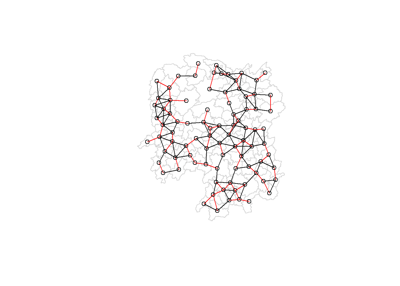

par(mfrow=c(1,2))
plot(hunan$geometry, border="lightgrey")
plot(k1, coords, add=TRUE, col="red", length=0.08, main="1st nearest neighbours")
plot(hunan$geometry, border="lightgrey")
plot(wm_d62, coords, add=TRUE, pch = 19, cex = 0.6, main="Distance link")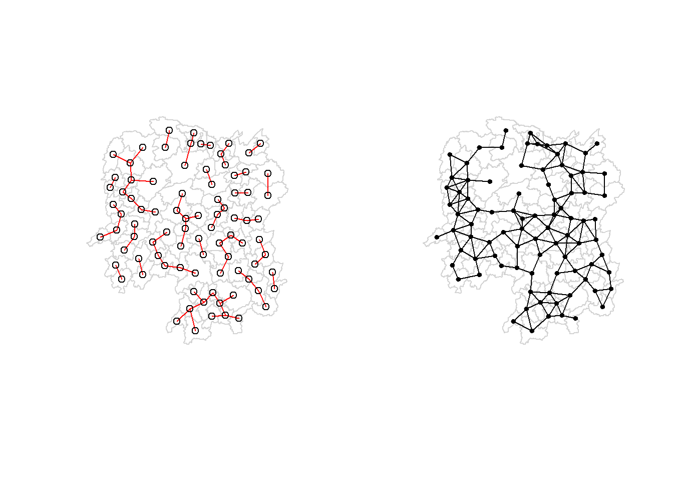

Computing adaptive distance weight matrix

knn6 <- knn2nb(knearneigh(coords, k=6))
knn6

Neighbour list object:
Number of regions: 88 
Number of nonzero links: 528 
Percentage nonzero weights: 6.818182 
Average number of links: 6 
Non-symmetric neighbours list

str(knn6)

List of 88
 $ : int [1:6] 2 3 4 5 57 64
 $ : int [1:6] 1 3 57 58 78 85
 $ : int [1:6] 1 2 4 5 57 85
 $ : int [1:6] 1 3 5 6 69 85
 $ : int [1:6] 1 3 4 6 69 85
 $ : int [1:6] 3 4 5 69 75 85
 $ : int [1:6] 9 66 67 71 74 84
 $ : int [1:6] 9 46 47 78 80 86
 $ : int [1:6] 8 46 66 68 84 86
 $ : int [1:6] 16 19 22 70 72 73
 $ : int [1:6] 10 14 16 17 70 72
 $ : int [1:6] 13 15 60 61 63 83
 $ : int [1:6] 12 15 60 61 63 83
 $ : int [1:6] 11 15 16 17 72 83
 $ : int [1:6] 12 13 14 17 60 83
 $ : int [1:6] 10 11 17 22 72 83
 $ : int [1:6] 10 11 14 16 72 83
 $ : int [1:6] 20 22 23 63 77 83
 $ : int [1:6] 10 20 21 73 74 82
 $ : int [1:6] 18 19 21 22 23 82
 $ : int [1:6] 19 20 35 74 82 86
 $ : int [1:6] 10 16 18 19 20 83
 $ : int [1:6] 18 20 41 77 79 82
 $ : int [1:6] 25 28 31 52 54 81
 $ : int [1:6] 24 28 31 33 54 81
 $ : int [1:6] 25 27 29 33 42 81
 $ : int [1:6] 26 29 30 37 42 81
 $ : int [1:6] 24 25 33 49 52 54
 $ : int [1:6] 26 27 37 42 43 81
 $ : int [1:6] 26 27 28 33 49 81
 $ : int [1:6] 24 25 36 39 40 54
 $ : int [1:6] 24 31 50 54 55 56
 $ : int [1:6] 25 26 28 30 49 81
 $ : int [1:6] 36 40 41 45 56 80
 $ : int [1:6] 21 41 46 47 80 82
 $ : int [1:6] 31 34 40 45 56 80
 $ : int [1:6] 26 27 29 42 43 44
 $ : int [1:6] 23 43 44 62 77 79
 $ : int [1:6] 25 40 42 43 44 81
 $ : int [1:6] 31 36 39 43 45 79
 $ : int [1:6] 23 35 45 79 80 82
 $ : int [1:6] 26 27 37 39 43 81
 $ : int [1:6] 37 39 40 42 44 79
 $ : int [1:6] 37 38 39 42 43 79
 $ : int [1:6] 34 36 40 41 79 80
 $ : int [1:6] 8 9 35 47 78 86
 $ : int [1:6] 8 21 35 46 80 86
 $ : int [1:6] 49 50 51 52 53 55
 $ : int [1:6] 28 33 48 51 52 54
 $ : int [1:6] 32 48 51 52 54 55
 $ : int [1:6] 28 48 49 50 52 54
 $ : int [1:6] 28 48 49 50 51 54
 $ : int [1:6] 48 50 51 52 55 75
 $ : int [1:6] 24 28 49 50 51 52
 $ : int [1:6] 32 48 50 52 53 75
 $ : int [1:6] 32 34 36 78 80 85
 $ : int [1:6] 1 2 3 58 64 68
 $ : int [1:6] 2 57 64 66 68 78
 $ : int [1:6] 12 13 60 61 87 88
 $ : int [1:6] 12 13 59 61 63 87
 $ : int [1:6] 12 13 60 62 63 87
 $ : int [1:6] 12 38 61 63 77 87
 $ : int [1:6] 12 18 60 61 62 83
 $ : int [1:6] 1 3 57 58 68 76
 $ : int [1:6] 58 64 66 67 68 76
 $ : int [1:6] 9 58 67 68 76 84
 $ : int [1:6] 7 65 66 68 76 84
 $ : int [1:6] 9 57 58 66 78 84
 $ : int [1:6] 4 5 6 32 75 85
 $ : int [1:6] 10 16 19 22 72 73
 $ : int [1:6] 7 19 73 74 84 86
 $ : int [1:6] 10 11 14 16 17 70
 $ : int [1:6] 10 19 21 70 71 74
 $ : int [1:6] 19 21 71 73 84 86
 $ : int [1:6] 6 32 50 53 55 69
 $ : int [1:6] 58 64 65 66 67 68
 $ : int [1:6] 18 23 38 61 62 63
 $ : int [1:6] 2 8 9 46 58 68
 $ : int [1:6] 38 40 41 43 44 45
 $ : int [1:6] 34 35 36 41 45 47
 $ : int [1:6] 25 26 28 33 39 42
 $ : int [1:6] 19 20 21 23 35 41
 $ : int [1:6] 12 13 15 16 22 63
 $ : int [1:6] 7 9 66 68 71 74
 $ : int [1:6] 2 3 4 5 56 69
 $ : int [1:6] 8 9 21 46 47 74
 $ : int [1:6] 59 60 61 62 63 88
 $ : int [1:6] 59 60 61 62 63 87
 - attr(*, "region.id")= chr [1:88] "1" "2" "3" "4" ...
 - attr(*, "call")= language knearneigh(x = coords, k = 6)
 - attr(*, "sym")= logi FALSE
 - attr(*, "type")= chr "knn"
 - attr(*, "knn-k")= num 6
 - attr(*, "class")= chr "nb"

Plotting distance based neighbours

plot(hunan$geometry, border="lightgrey")
plot(knn6, coords, pch = 19, cex = 0.6, add = TRUE, col = "red")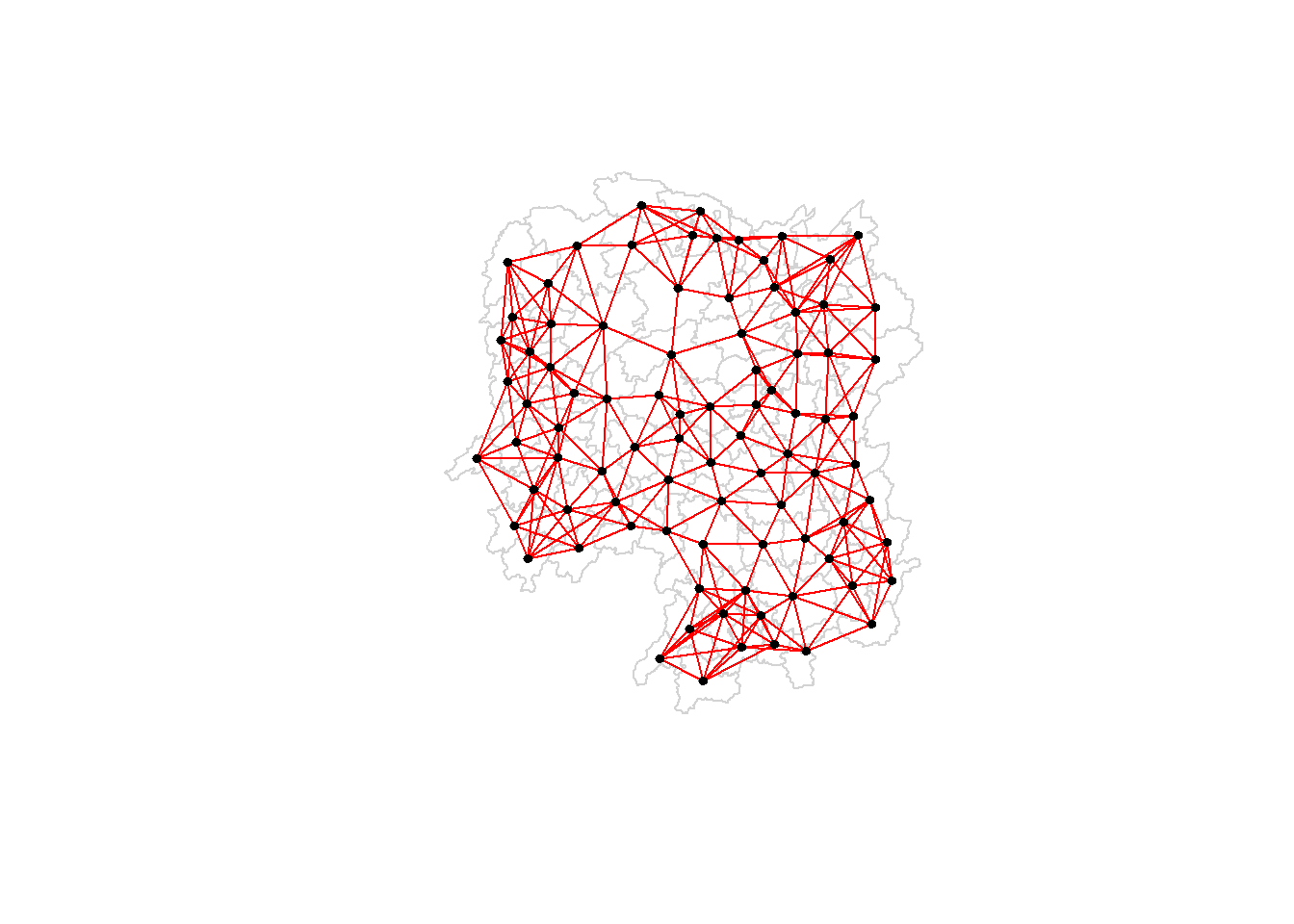

Weights based on IDW

dist <- nbdists(wm_q, coords, longlat = TRUE)
ids <- lapply(dist, function(x) 1/(x))
ids

[[1]]
[1] 0.01535405 0.03916350 0.01820896 0.02807922 0.01145113

[[2]]
[1] 0.01535405 0.01764308 0.01925924 0.02323898 0.01719350

[[3]]
[1] 0.03916350 0.02822040 0.03695795 0.01395765

[[4]]
[1] 0.01820896 0.02822040 0.03414741 0.01539065

[[5]]
[1] 0.03695795 0.03414741 0.01524598 0.01618354

[[6]]
[1] 0.015390649 0.015245977 0.021748129 0.011883901 0.009810297

[[7]]
[1] 0.01708612 0.01473997 0.01150924 0.01872915

[[8]]
[1] 0.02022144 0.03453056 0.02529256 0.01036340 0.02284457 0.01500600 0.01515314

[[9]]
[1] 0.02022144 0.01574888 0.02109502 0.01508028 0.02902705 0.01502980

[[10]]
[1] 0.02281552 0.01387777 0.01538326 0.01346650 0.02100510 0.02631658 0.01874863
[8] 0.01500046

[[11]]
[1] 0.01882869 0.02243492 0.02247473

[[12]]
[1] 0.02779227 0.02419652 0.02333385 0.02986130 0.02335429

[[13]]
[1] 0.02779227 0.02650020 0.02670323 0.01714243

[[14]]
[1] 0.01882869 0.01233868 0.02098555

[[15]]
[1] 0.02650020 0.01233868 0.01096284 0.01562226

[[16]]
[1] 0.02281552 0.02466962 0.02765018 0.01476814 0.01671430

[[17]]
[1] 0.01387777 0.02243492 0.02098555 0.01096284 0.02466962 0.01593341 0.01437996

[[18]]
[1] 0.02039779 0.02032767 0.01481665 0.01473691 0.01459380

[[19]]
[1] 0.01538326 0.01926323 0.02668415 0.02140253 0.01613589 0.01412874

[[20]]
[1] 0.01346650 0.02039779 0.01926323 0.01723025 0.02153130 0.01469240 0.02327034

[[21]]
[1] 0.02668415 0.01723025 0.01766299 0.02644986 0.02163800

[[22]]
[1] 0.02100510 0.02765018 0.02032767 0.02153130 0.01489296

[[23]]
[1] 0.01481665 0.01469240 0.01401432 0.02246233 0.01880425 0.01530458 0.01849605

[[24]]
[1] 0.02354598 0.01837201 0.02607264 0.01220154 0.02514180

[[25]]
[1] 0.02354598 0.02188032 0.01577283 0.01949232 0.02947957

[[26]]
[1] 0.02155798 0.01745522 0.02212108 0.02220532

[[27]]
[1] 0.02155798 0.02490625 0.01562326

[[28]]
[1] 0.01837201 0.02188032 0.02229549 0.03076171 0.02039506

[[29]]
[1] 0.02490625 0.01686587 0.01395022

[[30]]
[1] 0.02090587

[[31]]
[1] 0.02607264 0.01577283 0.01219005 0.01724850 0.01229012 0.01609781 0.01139438
[8] 0.01150130

[[32]]
[1] 0.01220154 0.01219005 0.01712515 0.01340413 0.01280928 0.01198216 0.01053374
[8] 0.01065655

[[33]]
[1] 0.01949232 0.01745522 0.02229549 0.02090587 0.01979045

[[34]]
[1] 0.03113041 0.03589551 0.02882915

[[35]]
[1] 0.01766299 0.02185795 0.02616766 0.02111721 0.02108253 0.01509020

[[36]]
[1] 0.01724850 0.03113041 0.01571707 0.01860991 0.02073549 0.01680129

[[37]]
[1] 0.01686587 0.02234793 0.01510990 0.01550676

[[38]]
[1] 0.01401432 0.02407426 0.02276151 0.01719415

[[39]]
[1] 0.01229012 0.02172543 0.01711924 0.02629732 0.01896385

[[40]]
[1] 0.01609781 0.01571707 0.02172543 0.01506473 0.01987922 0.01894207

[[41]]
[1] 0.02246233 0.02185795 0.02205991 0.01912542 0.01601083 0.01742892

[[42]]
[1] 0.02212108 0.01562326 0.01395022 0.02234793 0.01711924 0.01836831 0.01683518

[[43]]
[1] 0.01510990 0.02629732 0.01506473 0.01836831 0.03112027 0.01530782

[[44]]
[1] 0.01550676 0.02407426 0.03112027 0.01486508

[[45]]
[1] 0.03589551 0.01860991 0.01987922 0.02205991 0.02107101 0.01982700

[[46]]
[1] 0.03453056 0.04033752 0.02689769

[[47]]
[1] 0.02529256 0.02616766 0.04033752 0.01949145 0.02181458

[[48]]
[1] 0.02313819 0.03370576 0.02289485 0.01630057 0.01818085

[[49]]
[1] 0.03076171 0.02138091 0.02394529 0.01990000

[[50]]
[1] 0.01712515 0.02313819 0.02551427 0.02051530 0.02187179

[[51]]
[1] 0.03370576 0.02138091 0.02873854

[[52]]
[1] 0.02289485 0.02394529 0.02551427 0.02873854 0.03516672

[[53]]
[1] 0.01630057 0.01979945 0.01253977

[[54]]
[1] 0.02514180 0.02039506 0.01340413 0.01990000 0.02051530 0.03516672

[[55]]
[1] 0.01280928 0.01818085 0.02187179 0.01979945 0.01882298

[[56]]
[1] 0.01036340 0.01139438 0.01198216 0.02073549 0.01214479 0.01362855 0.01341697

[[57]]
[1] 0.028079221 0.017643082 0.031423501 0.029114131 0.013520292 0.009903702

[[58]]
[1] 0.01925924 0.03142350 0.02722997 0.01434859 0.01567192

[[59]]
[1] 0.01696711 0.01265572 0.01667105 0.01785036

[[60]]
[1] 0.02419652 0.02670323 0.01696711 0.02343040

[[61]]
[1] 0.02333385 0.01265572 0.02343040 0.02514093 0.02790764 0.01219751 0.02362452

[[62]]
[1] 0.02514093 0.02002219 0.02110260

[[63]]
[1] 0.02986130 0.02790764 0.01407043 0.01805987

[[64]]
[1] 0.02911413 0.01689892

[[65]]
[1] 0.02471705

[[66]]
[1] 0.01574888 0.01726461 0.03068853 0.01954805 0.01810569

[[67]]
[1] 0.01708612 0.01726461 0.01349843 0.01361172

[[68]]
[1] 0.02109502 0.02722997 0.03068853 0.01406357 0.01546511

[[69]]
[1] 0.02174813 0.01645838 0.01419926

[[70]]
[1] 0.02631658 0.01963168 0.02278487

[[71]]
[1] 0.01473997 0.01838483 0.03197403

[[72]]
[1] 0.01874863 0.02247473 0.01476814 0.01593341 0.01963168

[[73]]
[1] 0.01500046 0.02140253 0.02278487 0.01838483 0.01652709

[[74]]
[1] 0.01150924 0.01613589 0.03197403 0.01652709 0.01342099 0.02864567

[[75]]
[1] 0.011883901 0.010533736 0.012539774 0.018822977 0.016458383 0.008217581

[[76]]
[1] 0.01352029 0.01434859 0.01689892 0.02471705 0.01954805 0.01349843 0.01406357

[[77]]
[1] 0.014736909 0.018804247 0.022761507 0.012197506 0.020022195 0.014070428
[7] 0.008440896

[[78]]
[1] 0.02323898 0.02284457 0.01508028 0.01214479 0.01567192 0.01546511 0.01140779

[[79]]
[1] 0.01530458 0.01719415 0.01894207 0.01912542 0.01530782 0.01486508 0.02107101

[[80]]
[1] 0.01500600 0.02882915 0.02111721 0.01680129 0.01601083 0.01982700 0.01949145
[8] 0.01362855

[[81]]
[1] 0.02947957 0.02220532 0.01150130 0.01979045 0.01896385 0.01683518

[[82]]
[1] 0.02327034 0.02644986 0.01849605 0.02108253 0.01742892

[[83]]
[1] 0.023354289 0.017142433 0.015622258 0.016714303 0.014379961 0.014593799
[7] 0.014892965 0.018059871 0.008440896

[[84]]
[1] 0.01872915 0.02902705 0.01810569 0.01361172 0.01342099 0.01297994

[[85]]
 [1] 0.011451133 0.017193502 0.013957649 0.016183544 0.009810297 0.010656545
 [7] 0.013416965 0.009903702 0.014199260 0.008217581 0.011407794

[[86]]
[1] 0.01515314 0.01502980 0.01412874 0.02163800 0.01509020 0.02689769 0.02181458
[8] 0.02864567 0.01297994

[[87]]
[1] 0.01667105 0.02362452 0.02110260 0.02058034

[[88]]
[1] 0.01785036 0.02058034

Row-standardised weights matrix

rswm_q <- nb2listw(wm_q, style="W", zero.policy = TRUE)
rswm_q

Characteristics of weights list object:
Neighbour list object:
Number of regions: 88 
Number of nonzero links: 448 
Percentage nonzero weights: 5.785124 
Average number of links: 5.090909 

Weights style: W 
Weights constants summary:
   n   nn S0       S1       S2
W 88 7744 88 37.86334 365.9147

rswm_q$weights[10]

[[1]]
[1] 0.125 0.125 0.125 0.125 0.125 0.125 0.125 0.125

rswm_ids <- nb2listw(wm_q, glist=ids, style="B", zero.policy=TRUE)
rswm_ids

Characteristics of weights list object:
Neighbour list object:
Number of regions: 88 
Number of nonzero links: 448 
Percentage nonzero weights: 5.785124 
Average number of links: 5.090909 

Weights style: B 
Weights constants summary:
   n   nn       S0        S1     S2
B 88 7744 8.786867 0.3776535 3.8137

rswm_ids$weights[1]

[[1]]
[1] 0.01535405 0.03916350 0.01820896 0.02807922 0.01145113

summary(unlist(rswm_ids$weights))

    Min.  1st Qu.   Median     Mean  3rd Qu.     Max. 
0.008218 0.015088 0.018739 0.019614 0.022823 0.040338 

Application of Spatial Weight Matrix

Spatial lag with row-standardized weights

GDPPC.lag <- lag.listw(rswm_q, hunan$GDPPC)
GDPPC.lag

 [1] 24847.20 22724.80 24143.25 27737.50 27270.25 21248.80 43747.00 33582.71
 [9] 45651.17 32027.62 32671.00 20810.00 25711.50 30672.33 33457.75 31689.20
[17] 20269.00 23901.60 25126.17 21903.43 22718.60 25918.80 20307.00 20023.80
[25] 16576.80 18667.00 14394.67 19848.80 15516.33 20518.00 17572.00 15200.12
[33] 18413.80 14419.33 24094.50 22019.83 12923.50 14756.00 13869.80 12296.67
[41] 15775.17 14382.86 11566.33 13199.50 23412.00 39541.00 36186.60 16559.60
[49] 20772.50 19471.20 19827.33 15466.80 12925.67 18577.17 14943.00 24913.00
[57] 25093.00 24428.80 17003.00 21143.75 20435.00 17131.33 24569.75 23835.50
[65] 26360.00 47383.40 55157.75 37058.00 21546.67 23348.67 42323.67 28938.60
[73] 25880.80 47345.67 18711.33 29087.29 20748.29 35933.71 15439.71 29787.50
[81] 18145.00 21617.00 29203.89 41363.67 22259.09 44939.56 16902.00 16930.00

nb1 <- wm_q[[1]]
nb1 <- hunan$GDPPC[nb1]
nb1

[1] 20981 34592 24473 21311 22879

lag.list <- list(hunan$NAME_3, lag.listw(rswm_q, hunan$GDPPC))
lag.res <- as.data.frame(lag.list)
colnames(lag.res) <- c("NAME_3", "lag GDPPC")
hunan <- left_join(hunan,lag.res)

Joining, by = "NAME_3"

head(hunan)

Simple feature collection with 6 features and 36 fields
Geometry type: POLYGON
Dimension:     XY
Bounding box:  xmin: 110.4922 ymin: 28.61762 xmax: 112.3013 ymax: 30.12812
Geodetic CRS:  WGS 84
   NAME_2  ID_3  NAME_3   ENGTYPE_3 Shape_Leng Shape_Area  County    City
1 Changde 21098 Anxiang      County   1.869074 0.10056190 Anxiang Changde
2 Changde 21100 Hanshou      County   2.360691 0.19978745 Hanshou Changde
3 Changde 21101  Jinshi County City   1.425620 0.05302413  Jinshi Changde
4 Changde 21102      Li      County   3.474325 0.18908121      Li Changde
5 Changde 21103   Linli      County   2.289506 0.11450357   Linli Changde
6 Changde 21104  Shimen      County   4.171918 0.37194707  Shimen Changde
  avg_wage deposite     FAI Gov_Rev Gov_Exp     GDP GDPPC     GIO   Loan  NIPCR
1    31935   5517.2  3541.0  243.64  1779.5 12482.0 23667  5108.9 2806.9 7693.7
2    32265   7979.0  8665.0  386.13  2062.4 15788.0 20981 13491.0 4550.0 8269.9
3    28692   4581.7  4777.0  373.31  1148.4  8706.9 34592 10935.0 2242.0 8169.9
4    32541  13487.0 16066.0  709.61  2459.5 20322.0 24473 18402.0 6748.0 8377.0
5    32667    564.1  7781.2  336.86  1538.7 10355.0 25554  8214.0  358.0 8143.1
6    33261   8334.4 10531.0  548.33  2178.8 16293.0 27137 17795.0 6026.5 6156.0
   Bed    Emp  EmpR EmpRT Pri_Stu Sec_Stu Household Household_R NOIP Pop_R
1 1931 336.39 270.5 205.9  19.584  17.819     148.1       135.4   53 346.0
2 2560 456.78 388.8 246.7  42.097  33.029     240.2       208.7   95 553.2
3  848 122.78  82.1  61.7   8.723   7.592      81.9        43.7   77  92.4
4 2038 513.44 426.8 227.1  38.975  33.938     268.5       256.0   96 539.7
5 1440 307.36 272.2 100.8  23.286  18.943     129.1       157.2   99 246.6
6 2502 392.05 329.6 193.8  29.245  26.104     190.6       184.7  122 399.2
    RSCG Pop_T    Agri Service Disp_Inc      RORP    ROREmp lag GDPPC
1 3957.9 528.3 4524.41   14100    16610 0.6549309 0.8041262  24847.20
2 4460.5 804.6 6545.35   17727    18925 0.6875466 0.8511756  22724.80
3 3683.0 251.8 2562.46    7525    19498 0.3669579 0.6686757  24143.25
4 7110.2 832.5 7562.34   53160    18985 0.6482883 0.8312558  27737.50
5 3604.9 409.3 3583.91    7031    18604 0.6024921 0.8856065  27270.25
6 6490.7 600.5 5266.51    6981    19275 0.6647794 0.8407091  21248.80
                        geometry
1 POLYGON ((112.0625 29.75523...
2 POLYGON ((112.2288 29.11684...
3 POLYGON ((111.8927 29.6013,...
4 POLYGON ((111.3731 29.94649...
5 POLYGON ((111.6324 29.76288...
6 POLYGON ((110.8825 30.11675...

gdppc <- qtm(hunan, "GDPPC")
lag_gdppc <- qtm(hunan, "lag GDPPC")
tmap_arrange(gdppc, lag_gdppc, asp=1, ncol=2)

Spatial lag as a sum of neighboring values

b_weights <- lapply(wm_q, function(x) 0*x + 1)
b_weights2 <- nb2listw(wm_q, 
                       glist = b_weights, 
                       style = "B")
b_weights2

Characteristics of weights list object:
Neighbour list object:
Number of regions: 88 
Number of nonzero links: 448 
Percentage nonzero weights: 5.785124 
Average number of links: 5.090909 

Weights style: B 
Weights constants summary:
   n   nn  S0  S1    S2
B 88 7744 448 896 10224

lag_sum <- list(hunan$NAME_3, lag.listw(b_weights2, hunan$GDPPC))
lag.res <- as.data.frame(lag_sum)
colnames(lag.res) <- c("NAME_3", "lag_sum GDPPC")

lag_sum

[[1]]
 [1] "Anxiang"       "Hanshou"       "Jinshi"        "Li"           
 [5] "Linli"         "Shimen"        "Liuyang"       "Ningxiang"    
 [9] "Wangcheng"     "Anren"         "Guidong"       "Jiahe"        
[13] "Linwu"         "Rucheng"       "Yizhang"       "Yongxing"     
[17] "Zixing"        "Changning"     "Hengdong"      "Hengnan"      
[21] "Hengshan"      "Leiyang"       "Qidong"        "Chenxi"       
[25] "Zhongfang"     "Huitong"       "Jingzhou"      "Mayang"       
[29] "Tongdao"       "Xinhuang"      "Xupu"          "Yuanling"     
[33] "Zhijiang"      "Lengshuijiang" "Shuangfeng"    "Xinhua"       
[37] "Chengbu"       "Dongan"        "Dongkou"       "Longhui"      
[41] "Shaodong"      "Suining"       "Wugang"        "Xinning"      
[45] "Xinshao"       "Shaoshan"      "Xiangxiang"    "Baojing"      
[49] "Fenghuang"     "Guzhang"       "Huayuan"       "Jishou"       
[53] "Longshan"      "Luxi"          "Yongshun"      "Anhua"        
[57] "Nan"           "Yuanjiang"     "Jianghua"      "Lanshan"      
[61] "Ningyuan"      "Shuangpai"     "Xintian"       "Huarong"      
[65] "Linxiang"      "Miluo"         "Pingjiang"     "Xiangyin"     
[69] "Cili"          "Chaling"       "Liling"        "Yanling"      
[73] "You"           "Zhuzhou"       "Sangzhi"       "Yueyang"      
[77] "Qiyang"        "Taojiang"      "Shaoyang"      "Lianyuan"     
[81] "Hongjiang"     "Hengyang"      "Guiyang"       "Changsha"     
[85] "Taoyuan"       "Xiangtan"      "Dao"           "Jiangyong"    

[[2]]
 [1] 124236 113624  96573 110950 109081 106244 174988 235079 273907 256221
[11]  98013 104050 102846  92017 133831 158446 141883 119508 150757 153324
[21] 113593 129594 142149 100119  82884  74668  43184  99244  46549  20518
[31] 140576 121601  92069  43258 144567 132119  51694  59024  69349  73780
[41]  94651 100680  69398  52798 140472 118623 180933  82798  83090  97356
[51]  59482  77334  38777 111463  74715 174391 150558 122144  68012  84575
[61] 143045  51394  98279  47671  26360 236917 220631 185290  64640  70046
[71] 126971 144693 129404 284074 112268 203611 145238 251536 108078 238300
[81] 108870 108085 262835 248182 244850 404456  67608  33860

hunan <- left_join(hunan, lag.res)

Joining, by = "NAME_3"

gdppc <- qtm(hunan, "GDPPC")
lag_sum_gdppc <- qtm(hunan, "lag_sum GDPPC")
tmap_arrange(gdppc, lag_sum_gdppc, asp=1, ncol=2)

Spatial window average

wm_q1 <- wm_q

include.self(wm_q1)

Neighbour list object:
Number of regions: 88 
Number of nonzero links: 536 
Percentage nonzero weights: 6.921488 
Average number of links: 6.090909 

wm_q1 <- nb2listw(wm_q1)
wm_q1

Characteristics of weights list object:
Neighbour list object:
Number of regions: 88 
Number of nonzero links: 448 
Percentage nonzero weights: 5.785124 
Average number of links: 5.090909 

Weights style: W 
Weights constants summary:
   n   nn S0       S1       S2
W 88 7744 88 37.86334 365.9147

lag_w_avg_gpdpc <- lag.listw(wm_q1, 
                             hunan$GDPPC)
lag_w_avg_gpdpc

 [1] 24847.20 22724.80 24143.25 27737.50 27270.25 21248.80 43747.00 33582.71
 [9] 45651.17 32027.62 32671.00 20810.00 25711.50 30672.33 33457.75 31689.20
[17] 20269.00 23901.60 25126.17 21903.43 22718.60 25918.80 20307.00 20023.80
[25] 16576.80 18667.00 14394.67 19848.80 15516.33 20518.00 17572.00 15200.12
[33] 18413.80 14419.33 24094.50 22019.83 12923.50 14756.00 13869.80 12296.67
[41] 15775.17 14382.86 11566.33 13199.50 23412.00 39541.00 36186.60 16559.60
[49] 20772.50 19471.20 19827.33 15466.80 12925.67 18577.17 14943.00 24913.00
[57] 25093.00 24428.80 17003.00 21143.75 20435.00 17131.33 24569.75 23835.50
[65] 26360.00 47383.40 55157.75 37058.00 21546.67 23348.67 42323.67 28938.60
[73] 25880.80 47345.67 18711.33 29087.29 20748.29 35933.71 15439.71 29787.50
[81] 18145.00 21617.00 29203.89 41363.67 22259.09 44939.56 16902.00 16930.00

lag.list.wm_q1 <- list(hunan$NAME_3, lag.listw(wm_q1, hunan$GDPPC))
lag_wm_q1.res <- as.data.frame(lag.list.wm_q1)
colnames(lag_wm_q1.res) <- c("NAME_3", "lag_window_avg GDPPC")

hunan <- left_join(hunan, lag_wm_q1.res)

Joining, by = "NAME_3"

gdppc <- qtm(hunan, "GDPPC")
w_avg_gdppc <- qtm(hunan, "lag_window_avg GDPPC")
tmap_arrange(gdppc, w_avg_gdppc, asp=1, ncol=2)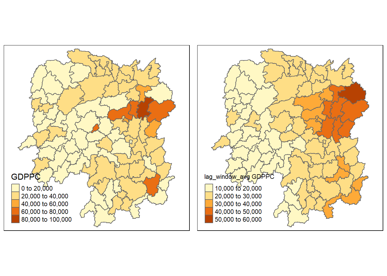

Spatial window sum

wm_q1 <- wm_q

include.self(wm_q1)

Neighbour list object:
Number of regions: 88 
Number of nonzero links: 536 
Percentage nonzero weights: 6.921488 
Average number of links: 6.090909 

wm_q1

Neighbour list object:
Number of regions: 88 
Number of nonzero links: 448 
Percentage nonzero weights: 5.785124 
Average number of links: 5.090909 

b_weights <- lapply(wm_q1, function(x) 0*x + 1)
b_weights[1]

[[1]]
[1] 1 1 1 1 1

b_weights2 <- nb2listw(wm_q1, 
                       glist = b_weights, 
                       style = "B")
b_weights2

Characteristics of weights list object:
Neighbour list object:
Number of regions: 88 
Number of nonzero links: 448 
Percentage nonzero weights: 5.785124 
Average number of links: 5.090909 

Weights style: B 
Weights constants summary:
   n   nn  S0  S1    S2
B 88 7744 448 896 10224

w_sum_gdppc <- list(hunan$NAME_3, lag.listw(b_weights2, hunan$GDPPC))
w_sum_gdppc

[[1]]
 [1] "Anxiang"       "Hanshou"       "Jinshi"        "Li"           
 [5] "Linli"         "Shimen"        "Liuyang"       "Ningxiang"    
 [9] "Wangcheng"     "Anren"         "Guidong"       "Jiahe"        
[13] "Linwu"         "Rucheng"       "Yizhang"       "Yongxing"     
[17] "Zixing"        "Changning"     "Hengdong"      "Hengnan"      
[21] "Hengshan"      "Leiyang"       "Qidong"        "Chenxi"       
[25] "Zhongfang"     "Huitong"       "Jingzhou"      "Mayang"       
[29] "Tongdao"       "Xinhuang"      "Xupu"          "Yuanling"     
[33] "Zhijiang"      "Lengshuijiang" "Shuangfeng"    "Xinhua"       
[37] "Chengbu"       "Dongan"        "Dongkou"       "Longhui"      
[41] "Shaodong"      "Suining"       "Wugang"        "Xinning"      
[45] "Xinshao"       "Shaoshan"      "Xiangxiang"    "Baojing"      
[49] "Fenghuang"     "Guzhang"       "Huayuan"       "Jishou"       
[53] "Longshan"      "Luxi"          "Yongshun"      "Anhua"        
[57] "Nan"           "Yuanjiang"     "Jianghua"      "Lanshan"      
[61] "Ningyuan"      "Shuangpai"     "Xintian"       "Huarong"      
[65] "Linxiang"      "Miluo"         "Pingjiang"     "Xiangyin"     
[69] "Cili"          "Chaling"       "Liling"        "Yanling"      
[73] "You"           "Zhuzhou"       "Sangzhi"       "Yueyang"      
[77] "Qiyang"        "Taojiang"      "Shaoyang"      "Lianyuan"     
[81] "Hongjiang"     "Hengyang"      "Guiyang"       "Changsha"     
[85] "Taoyuan"       "Xiangtan"      "Dao"           "Jiangyong"    

[[2]]
 [1] 124236 113624  96573 110950 109081 106244 174988 235079 273907 256221
[11]  98013 104050 102846  92017 133831 158446 141883 119508 150757 153324
[21] 113593 129594 142149 100119  82884  74668  43184  99244  46549  20518
[31] 140576 121601  92069  43258 144567 132119  51694  59024  69349  73780
[41]  94651 100680  69398  52798 140472 118623 180933  82798  83090  97356
[51]  59482  77334  38777 111463  74715 174391 150558 122144  68012  84575
[61] 143045  51394  98279  47671  26360 236917 220631 185290  64640  70046
[71] 126971 144693 129404 284074 112268 203611 145238 251536 108078 238300
[81] 108870 108085 262835 248182 244850 404456  67608  33860

w_sum_gdppc.res <- as.data.frame(w_sum_gdppc)
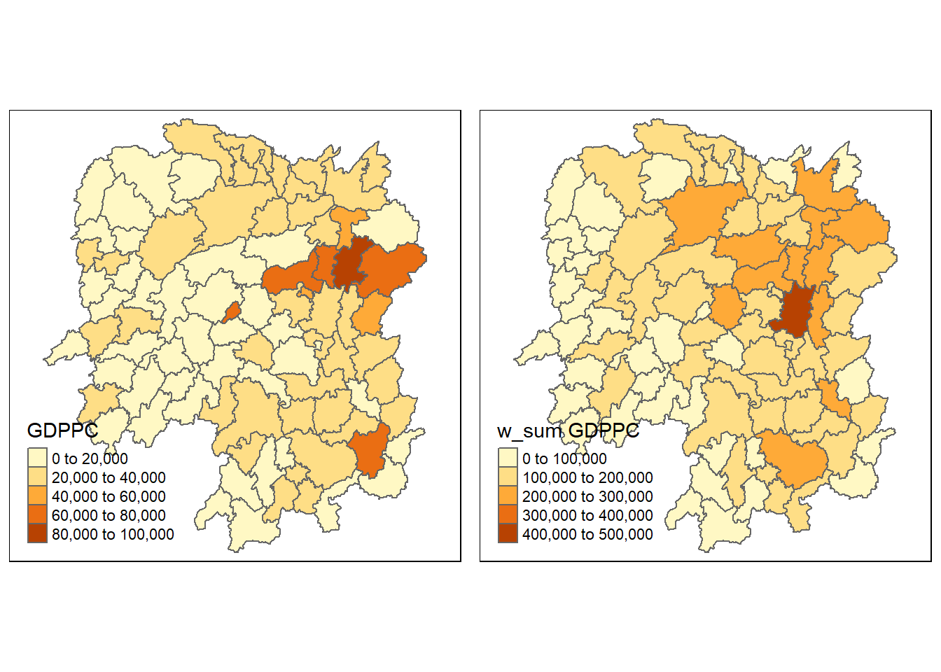
colnames(w_sum_gdppc.res) <- c("NAME_3", "w_sum GDPPC")

hunan <- left_join(hunan, w_sum_gdppc.res)

Joining, by = "NAME_3"

gdppc <- qtm(hunan, "GDPPC")
w_sum_gdppc <- qtm(hunan, "w_sum GDPPC")
tmap_arrange(gdppc, w_sum_gdppc, asp=1, ncol=2)